

Figure
1.
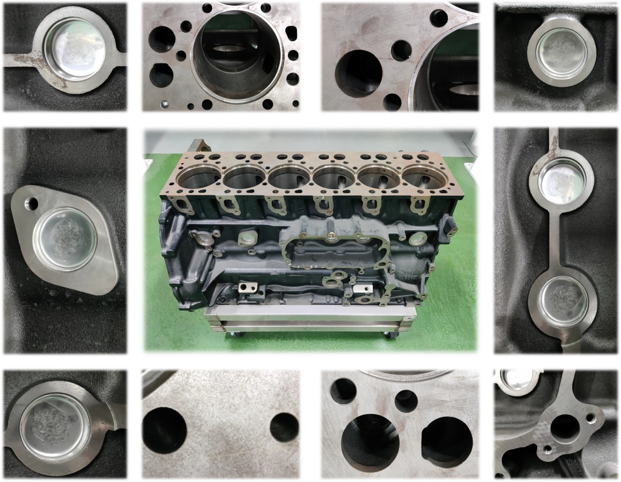
The surface structural characteristics of castings, using an engine as the example.

IEEE/CAA Journal of Automatica Sinica
| Citation: | K. Mao, P. Wei, Y. Wang, M. Liu, S. Wang, and N. Zheng, “CSDD: A benchmark dataset for casting surface defect detection and segmentation,” IEEE/CAA J. Autom. Sinica, vol. 12, no. 5, pp. 1–13, May 2025.

|
SURFACE defect detection is an essential step in industrial production as surface defects have adverse effects on the quality of industrial products, especially for the casting production. Traditional manual inspection manners are time-consuming and labor-intensive, leading to inconsistent and unreliable defect detection results. Automated surface defect detection instruments are crucial as they offer high efficiency, consistency and accuracy, enabling timely identification of defects. Most automated surface defect detection instruments first capture images of industrial products using visual sensors, and then use various algorithms to detect defects. High-precision defect detection methods play an important role in these instruments.
Nowadays, defect detection methods using deep learning models has been receiving growing research attention [1]–[12]. While these methods have achieved remarkable progress, casting surface defect detection has still considerable room for improvement. Lack of sufficient and high-quality data has become one of the most challenging problems. Developing methods for casting surface defect detection requires substantial defect data. However, extant datasets [13]–[19] are characterized by inherent limitations, including low image resolution, simple background structure, constrained data volume, etc. There is an urgent need for a benchmark dataset that better aligns with real-world industrial production conditions.
Collecting defective samples in industrial scenes is a challenging task. This is because, in many situations, the vast majority of products produced during the manufacturing process are defect-free. The probability of encountering a defective sample is extremely low, with some defects only appearing once every few months. This makes it challenging to gather a large number of defective samples.
Castings are a significant category of industrial products and widely used in various industries, as depicted in Fig. 1. During the production or usage process, the casting surface may exhibit various defects, such as cracks, shrinkage cavities and inclusions, which significantly impact the performance and compromise the mechanical properties.
In this paper, we build a benchmark Casting Surface Defect Dataset (CSDD). The dataset contains
We conduct a comprehensive series of comparative experiments, leveraging well-established detection and segmentation methods to rigorously compare the performance of various methods. Moreover, we propose a new defect detection method by integrating the global attention mechanism and partial convolution into YOLOv5 [20]. Experimental results demonstrate that the proposed method significantly improves the defect detection performance.
Our contributions are summarized as follows.
1) We construct a casting surface defect dataset, which can serve as a novel benchmark for casting surface defect detection and segmentation.
2) We extensively evaluate existing methods of defect detection and segmentation on the CSDD, providing comprehensive baselines for future research.
3) We propose a defect detection method that incorporates the global attention mechanism and partial convolution, further improving the detection performance.
Datasets with sufficient samples are vital for surface defect detection. Collecting defective samples is a nontrivial task since most samples in industrial production are products without defects. For this reason, the scale, diversity, and amounts of existing defect datasets are inferior to the general object detection datasets. Nevertheless, many studies have striven to build reasonable defect datasets and achieved considerable progress over the past decade.
NEU-DET [13] comprises
BSData [16] collects
The above datasets contribute greatly to the research community and industrial applications. However, a common limitation is that the images in these datasets either have simple inner structures or smooth textures, which make the defects more distinct. Our CSDD is larger in scale than most existing datasets. More importantly, our images feature complex inner structures and backgrounds that intertwine with the defects, presenting significant challenges for defect detection and segmentation.
Object detection aims to identify and localize objects within an image, using algorithms to classify each object and predict its bounding box. Recently, deep learning-based object detection methods [20]–[28] have garnered significant attention due to their superior accuracy and robustness. These methods can also be applied to defect detection, enabling the identification of defects in various materials and products with high precision.
Faster RCNN [21] is a classic two-stage object detection method. It consists of a feature extractor, a region proposal network and an object classifier. Faster RCNN can achieve high accuracy, but the prediction speed is slower compared to one-stage object detection methods. One the basis of Faster RCNN, Cascade RCNN [22] adopts a cascaded detector and RPN structure. It improves the detection accuracy and robustness, but the training time and computing resource requirement also increase accordingly.
SSD [23] is a one-stage object detection method and can realize the detection of multi-scale objects by predicting on feature maps at different scales. Compared to other methods, SSD is faster and has a better performance on small objects. However, it has disadvantages in detecting large objects and dealing with the issue of class imbalance between positive and negative samples. On the basis of SSD, RetinaNet [24] proposes focal loss to solve the problem of class imbalance between positive and negative samples. It performs better in dealing with the problem of class imbalance, but the detection accuracy is relatively low.
YOLOv5 [20] consists of two parts: a feature extraction network and a detection network. Compared with other object detection models, YOLOv5 has a faster detection speed. But it faces challenges in detecting small objects and overlapped ones. YOLOv8 [29], building on the foundation of YOLOv5, incorporates a more advanced backbone and an anchor-free head, further enhancing the efficiency of detection. YOLOv10 [30] introduces consistent dual assignments for NMS-free training and a holistic efficiency-accuracy driven model design strategy to better achieve real-time object detection. CenterNet [25] detects objects by classifying center points and regressing bounding boxes on feature maps at different scales, which has advantages in both speed and accuracy. However, it faces challenges in detecting small objects and handing overlapped ones. FCOS [26] represents a fully convolutional, single-stage object detection framework. It facilitates efficient detection for multi-scale objects. This approach obviates the necessity for intricate anchor box design and sample selection stages inherent in conventional object detection methodologies.
Deformable DETR [27] is a variant of DETR [31] object detection method, which improves the detection performance through the incorporation of a deformable attention mechanism. It enhances the precision and adaptability of feature representations. Conditional DETR [28] learns conditional spatial queries from embeddings in the decoder and implements a multi-head cross-attention mechanism, which achieves faster convergence than conventional DETR [31].
In recent years, surface defect detection has received more and more attention for its importance to industrial production. Many researchers have studied this problem and proposed impressive approaches.
Traditional methods extract hand-crafted features from images and use statistical learning methods to detect surface defects. Tsanakas et al. [32] utilize edge detection operators for operating photovoltaic modules. Yuan et al. [33] introduce a thresholding method for defect detection based on the otsu algorithm [34]. Li and Tsai [35] propose an automatic visual inspection method based on Fourier image reconstruction. Cen et al. [36] propose a defect inspection method for defect inspection of TFT-LCD panels based on low-rank matrix model. Jian et al. [37] propose a method for detecting possible defects in the manufacturing process of mobile phone screens. They employ a contour-based registration method to generate template images for aligning the images.
However, these traditional methods rely on hand-crafted features, which are less effective in complex environments or with intricate defects.
Recently, many researchers apply deep learning methods to defect detection. SDDNet [7] integrates a feature retaining block to preserve texture information and a skip densely connected module to propagate fine-grained details for improved prediction of defects. Zeng et al. [38] present the atrous spatial pyramid pooling-balanced-feature pyramid network, a novel feature fusion method for enhancing small object detection, particularly validated on tiny defect detection in printed circuit boards. Jain et al. [39] introduce a framework employing Generative Adversarial Networks for synthetic data augmentation, significantly boosting the surface defect detection performance. Wang et al. [9] introduce a novel method for surface defect detection by integrating global context-based self-similarity feature augmentation with a multi-scale bidirectional feature fusion module. ETDNet [10] incorporates a lightweight vision transformer, a channel-modulated feature pyramid network and a task-oriented decoupled head to improve classification and regression task performance. Li et al. [11] propose a method for detecting micro-defects on printed circuit board assemblies, which integrates a semantic segmentation network with rule-based detection algorithms. An improved YOLOv5 model based on the Wasserstein GAN algorithm is proposed for small sample defect detection by Han et al. [12].
While the above existing approaches have made great progress in defect detection, there is still considerable room for improvement for the challenges of inner structure influence, illumination changes and defect shape variance. To overcome these problems, we propose an improved method with the global attention mechanism and partial convolution.
Semantic segmentation methods can be broadly categorized into two main classes: CNN-based methods and Transformer-based methods.
1) CNN-Based Methods: FCN [40] replaces fully connected layers with fully convolutional layers, enabling pixel-wise segmentation. UNet [41] employs a U-shaped encoder-decoder structure with skip connections. The skip connections facilitate the fusion of low-level and high-level features, enabling precise segmentation of objects and achieving remarkable segmentation accuracy. DeepLabv3 [42] employs atrous convolution in cascade or in parallel to capture multi-scale context by adopting multiple atrous rate and significantly improves their previous DeepLab versions [43] without DenseCRF post-processing. DeepLabv3plus [44] adds a decoder module to refine the segmentation results based on [42] and apply the depth wise separable convolution to both Atrous Spatial Pyramid Pooling and decoder modules. FastFCN [45] introduces the Joint Pyramid Upsampling module to replace dilated convolutions, reducing computation complexity by over three times without performance loss. CGNet [46] is a lightweight and efficient semantic segmentation. It introduces the Context Guided block to capture joint features of local and global contexts, enhancing the segmentation accuracy. DDRNet [47] proposes a family of efficient backbones specially designed for real-time semantic segmentation, achieving an impressive balance between accuracy and speed. PIDNet [48] is an innovative three-branch network for real-time semantic segmentation, combining detail, context, and boundary information for high accuracy and speed.
2) Transformer-Based Methods: Segmenter [49] extends the Vision Transformer (ViT) to semantic segmentation, utilizing output embeddings of image patches and employing either a point-wise linear decoder or a mask transformer decoder for class label prediction. SegFormer [50] introduces a novel hierarchically structured transformer encoder, generating multi-scale features without positional encoding. It achieves significantly better performance and efficiency compared to previous methods. MaskFormer [51] is a novel semantic and instance level segmentation method that predicts a set of binary masks, each associated with a single global class label, handling semantic and panoptic segmentation tasks in a unified manner. Mask2Former [52] employs the masked attention to extract localized features within predicted mask regions, further enhancing the performance.
Since there was no suitable dataset for casting surface defects with complex casting structures, we have created a new Casting Surface Defect Dataset. We believe this dataset will benefit both the industrial vision research and manufacturing applications.
In practical production processes, most samples are defect-free, making it challenging to collect a sufficient number of defective samples. To overcome this problem, we adopt a manufacturing-simulation approach for defective data collection.
Firstly, we machine a large number of metal plates, each measuring 30 centimeters in length and width. We design the surface structures based on actual castings, such as automotive engines shown in Fig. 1. Then, we use machines to create more than ten cavities of different sizes and layouts on each metal plate. The radius of these cavities ranges from 0.4 to 4 centimeters. These metal plates with cavities are intended to simulate the actual casting surfaces, such as those found in automotive engines.
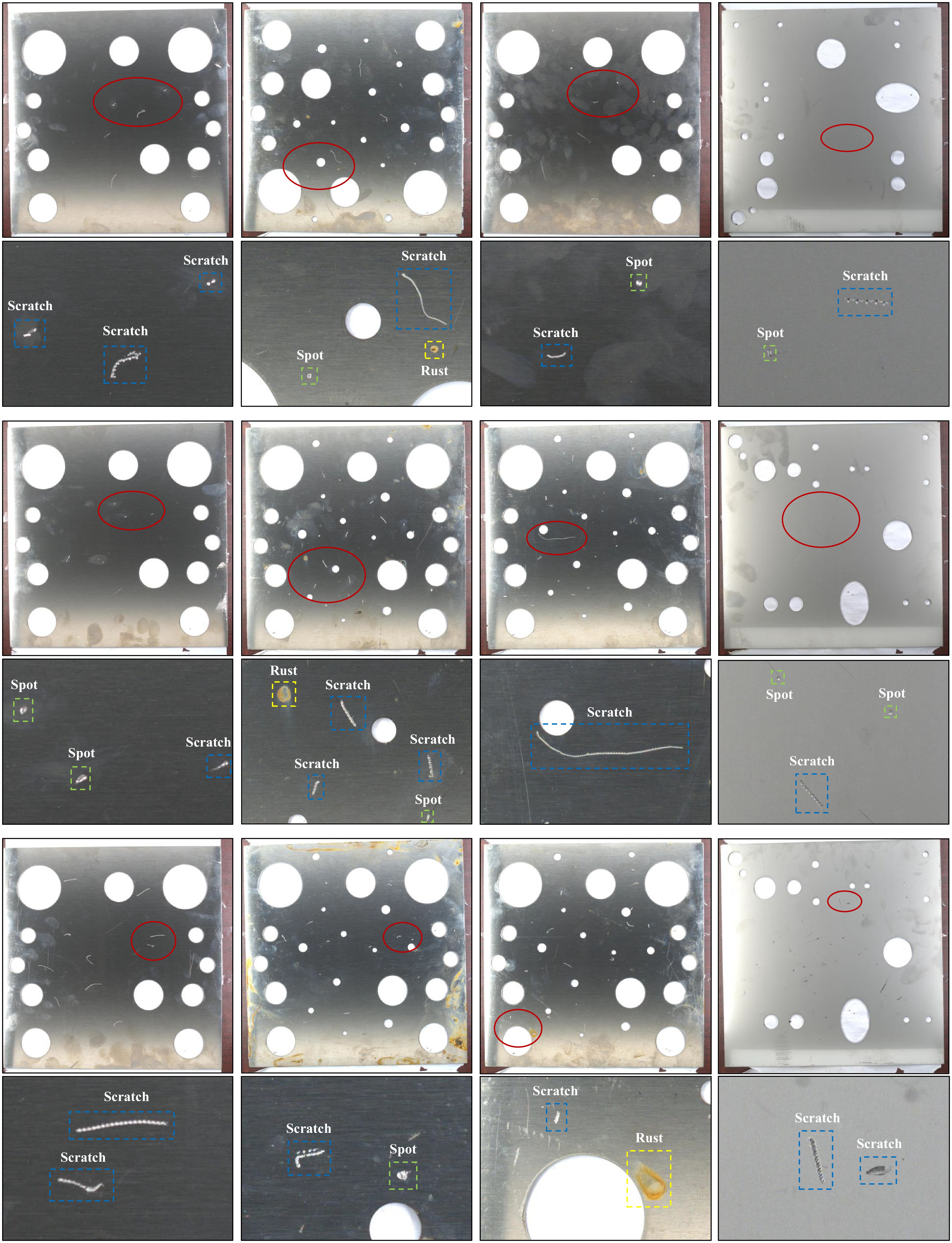
Secondly, we use production tools to create defects on the metal plates, including three types: scratches, spots and rusts. The sizes of these defects could be very small and vary significantly. To ensure that the casting surface and defects closely resemble those found in practical products, we produce them under the instructions of professional production and quality inspection engineers.
Finally, the metal plates are captured using a visual sensor. We manually annotate each image with the defect type and the corresponding defect region. For the annotation of the CSDD, we first randomly divide the images into six groups of approximately equal size, with each group assigned to an independent annotator who labels the defects in each image. After completing this process, each annotator double-checks and amends the annotations made by the other five annotators to ensure the accuracy and consistency of the labels.
Due to the reflective nature of metal plates, it is extremely difficult to obtain uniform illumination images. In this case, we carefully design an imaging scheme. We use four strip lights to surround and illuminate the metal plates. Meanwhile, the intensity and angle of these strip lights can be adjusted to capture the highest quality images. Besides, in order to obtain images with uniform brightness, we use the gamma correction to process the captured images. After adjusting the exposure time and gain, we successfully obtain images with uniform illumination.
Through these procedures, the Casting Surface Defect Dataset are built. It contains
| Dataset | Objects | Structure | Images | Anno. images | Anno. defects | Color mode | Resolution | Anno. type | Defect types |
| NEU-DET [13] | Steel Strip | 200×200 | Bbox | 6 | |||||
| GC10-DET [17] | Metal | 2048×1000 | Bbox | 10 | |||||
| Severstal [19] | Steel | 18074 | 12568 | 1600×256 | Pixel | 4 | |||
| KolektorSDD [14] | Commutator | 399 | 399 | 56 | 1270×500 | Pixel | 1 | ||
| KolektorSDD2 [15] | Commutator | 394 | √ | 649×241 | Pixel | 1 | |||
| SD-saliency-900 [18] | Steel Strip | 900 | 900 | 200×200 | Pixel | 3 | |||
| BSData [16] | Spindle | √ | 485 | √ | 2816×1016 | Pixel | 1 | ||
| CSDD(Ours) | Casting | √ | √ | 3648×3648 | Pixel | 3 |
 DownLoad:
CSV
DownLoad:
CSV
| Type | Number | Width (Avg) | Height (Avg) |
| Scratch | 71.77 | 39.23 | |
| Spot | 24.40 | 20.83 | |
| Rust | 71.55 | 41.34 |
DownLoad:
CSV
The comparison between our CSDD and the existing datasets introduced in Section II-A is depicted in Table I and Fig. 3. In comparison to the existing datasets, our CSDD demonstrates several notable complexities.
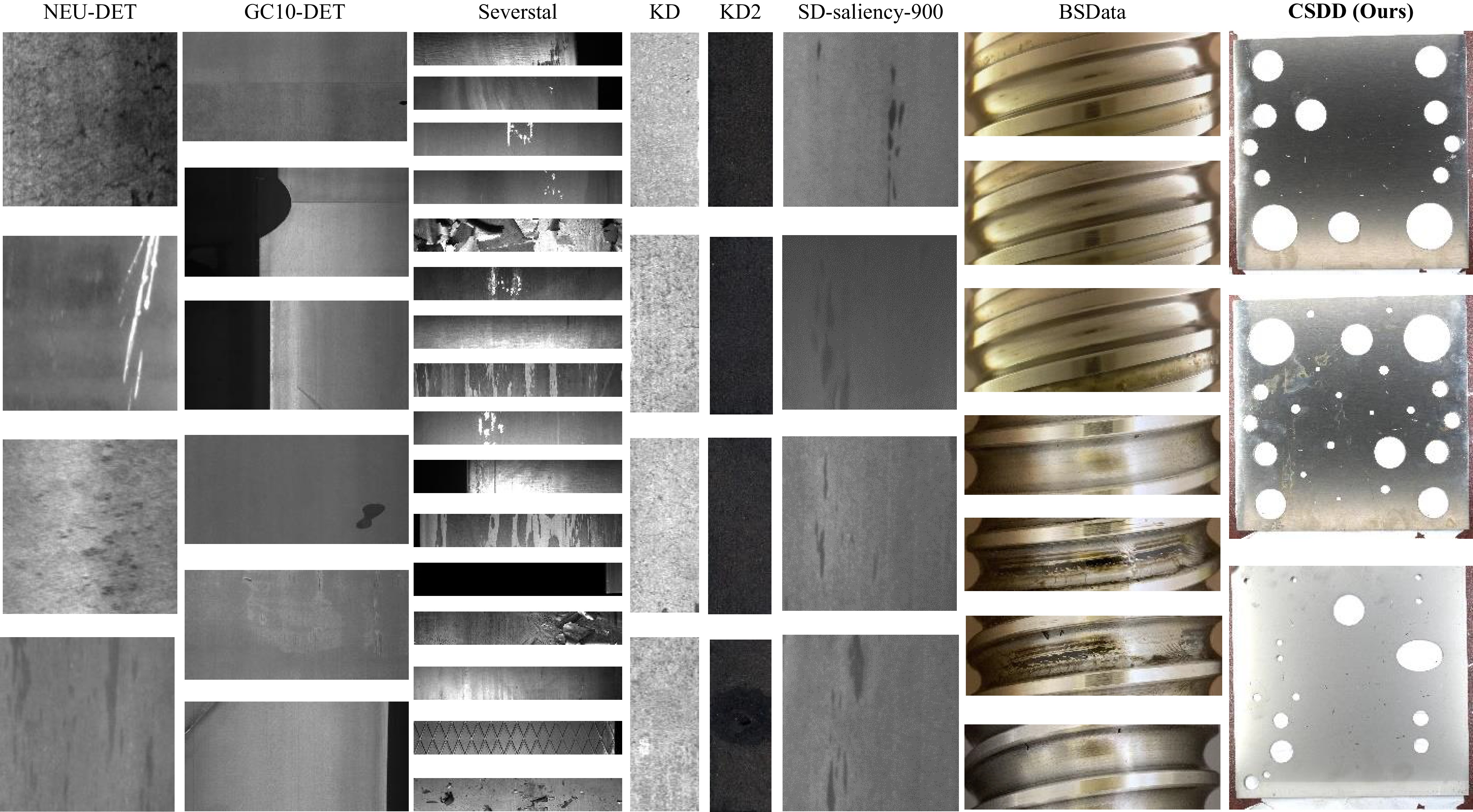
First, it has a large number of images and defects. As shown in Table I, our CSDD has
Second, the images in our CSDD have complex inner structures. These inner structures would disturb the defect detection and makes the task more challenging, as shown in Fig. 2, which are closer to the practical applications.
Besides, the size of the defect is extremely small compared to the size of the image, as shown in Fig. 2. The size of the casting surface in our CSDD is 30 centimeters long while the sizes of some defects are smaller than 0.1 centimeters. The image resolution is 3648×3648, while most defects are smaller than 100 pixels, with some even less than 50 pixels. This significant difference in size presents challenges associated with detecting “small objects”.
In this section, we present an method for defect detection by incorporating the global attention mechanism and partial convolution into YOLOv5 [20]. The method, along with the approaches introduced in Section II-B, can serve as baselines for defect detection on our CSDD.
We enhance the standard YOLOv5[20] by incorporating both the global attention mechanism (GAM) [53] and partial convolution (PConv) [54]. The overall architecture is depicted in Fig. 4. The convolution (Conv), bottleneck with 3 convolutions (C3), spatial pyramid pooling (SPPF), upsample, and detect modules remain consistent with the standard YOLOv5 [4]. We incorporate GAM preceding the SPPF module and substitute two of the C3 modules with P3 modules in the backbone part. We will provide detailed introductions to GAM and P3 in Sections IV-B and IV-C, respectively.

As shown in Fig. 4, our model comprises three main components: the backbone, the neck and the head. The backbone functions as the feature extractor, utilizing Conv, C3, P3, GAM and SPPF to extract features from the input images. The Conv module is primarily used for downsampling the input, while the C3 module performs feature extraction and fusion to obtain feature maps containing rich semantic information. The SPPF module further enhances the semantic information contained in the deepest feature maps through pooling and feature fusion. We replace two C3 modules in the standard YOLOv5 with two P3 modules and add a GAM module before the SPPF module. The neck integrates feature maps of three different scales extracted from various stages of the backbone. By merging shallow features, it ensures that the resulting feature maps possess both rich semantic information and precise positional details. The head conducts predictions on the feature maps of three different scales obtained from the neck, and consolidates the prediction results to form the final detection outcome.
Attention mechanisms can effectively enhance the representational capacity of feature maps, thereby contributing to detection tasks. The Convolutional Block Attention Module (CBAM) [55] sequentially infers attention maps along channel and spatial dimensions, then utilizes these attention maps to adaptively refine feature maps. The global attention mechanism [53] redesigns the sequential channel-spatial attention mechanism from CBAM and achieves better performance. We use the global attention mechanism [53] in our method to enhance the model’s ability to perceive defect details, thereby improving its detection performance.
Given the input feature map F1, it sequentially passes through the channel attention module and the spatial attention module. The intermediate state F2 and the output F3 are defined as
| F2=Mc(F1)⊗F1 | (1) |
| F3=Ms(F2)⊗F2 | (2) |
where ⊗ denotes element-wise multiplication, Mc is the channel attention submodule and Ms is the spatial attention submodule. The channel attention submodule of GAM employs 3D permutation, while the spatial attention submodule utilizes two convolutional layers for spatial information fusion.
Fast neural networks with low latency and high throughput are crucial, especially for neural networks deployed in real-world scenarios. PConv [54] applies a regular convolution to only a portion of the input channels, leaving the rest untouched. Building upon PConv, fast neural network (FasterNet) [54] achieves the state-of-the-art performance in classification and detection tasks, with significantly lower latency and higher throughput.
We make modifications to the C3 module of the standard YOLOv5 [20], as illustrated in Fig. 5. The conv, bn and relu represent the standard convolution, batch normalization and relu operation, respectively. We name the modified C3 module as the P3 module. The P3 module comprises three FasterNet Blocks [54], with each FasterNet Block containing a PConv.

We incorporate GAM preceding the SPPF module and substitute two of the C3 modules with P3 in the backbone part. With GAM, the model becomes more adept at capturing features specific to defects themselves, thereby aiding downstream detection tasks. Through the integration of PConv, the model further enhances detection performance while maintaining a reduced parameter count.
In this section, we perform a comprehensive evaluation of several state-of-the-art methods for defect detection and segmentation on our CSDD, respectively. We also evaluate the method proposed in this paper and compare it with other approaches. These results can serve as baselines for future research.
The CSDD contains
For defect detection, we use the average precision (AP) and the mean average precision (mAP) as the evaluation metrics. They are defined as follows:
| Precision=TPbboxTPbbox+FPbboxRecall=TPbboxTPbbox+FNbbox | (3) |
where TPbbox, FPbbox and FNbbox are the number of true positives, false positives and false negatives, at the bounding box level. The AP is computed as the area under the precision-recall curve, while the mAP represents the average AP across all defect types.
For defect segmentation, the Intersection over Union (IoU) and mean Intersection over Union (mIoU) are used as the evaluation metrics. The IoU is defined as follows:
| IoU=TPpixelTPpixel+FPpixel+FNpixel | (4) |
where TPpixel, FPpixel and FNpixel are the number of true positives, false positives and false negatives, at the pixel level. The mIoU is the mean value of the IoU across all defect types.
Additionally, we utilize giga floating point operations (GFLOPs) [56] to evaluate the complexity of different methods for both defect detection and segmentation. GFLOPs quantifies the total number of floating-point operations required for a single forward pass. A lower GFLOPs indicates a lower complexity of the method.

For defect detection, we implement the CNN-based and Transformer-based methods mentioned in Section II-B using MMDetection [56], excluding YOLOv5, YOLOv8 and YOLOv10. For YOLOv5, YOLOv8 and YOLOv10, we utilize their official open-source project packages [20], [29], [30]. Most experimental parameters are kept consistent with the default parameters in MMDetection. For image augmentation, we employ the default configurations from MMDetection [56]. In order to make the object detection methods based on Transformer architecture have scale invariance and stronger generalization ability, data enhancement methods including random choice resize are widely used in MMDetection [56]. The input size of Transformer-based methods is a dynamically changing range. Therefore, we follow the default settings in MMDetection[56] without forcing all image inputs to be scaled to 1024×1024. We use 4 NVIDIA Tesla
| Methods | Optimizer | Learning rate | Weight decay | Momentum | Augmentation | Loss | Scheduler | Batch size | Epochs |
| Faster R-CNN [21] | SGD | 0.02 | 0.9 | Random flip | L1 loss (bbox) CE loss (cls) | Linear LR | 4 | 48 | |
| Cascade R-CNN [22] | SGD | 0.02 | 0.9 | Random flip | Smooth L1 loss (bbox) CE loss (cls) |
Linear LR | 4 | 48 | |
| SSD [23] | SGD | 0.002 | 0.9 | Random crop Random flip |
Smooth L1 loss (bbox) CE loss (cls) |
Linear LR | 4 | 48 | |
| RetinaNet [24] | SGD | 0.02 | 0.9 | Random flip | L1 loss (bbox) Focal loss (cls) |
Linear LR | 4 | 48 | |
| YOLOv5 [20] | SGD | 0.01 | 0.8 | Mosaic, mixup HSV color-space random flip |
CIoU loss (location) BCE loss (class+object) |
Lambda LR | 4 | 300 | |
| YOLOv8 [29] | SGD | 0.01 | 0.8 | Mosaic, mixup HSV color-space random flip |
CIoU loss (location) BCE loss (class+object) |
Lambda LR | 4 | 300 | |
| YOLOv10 [30] | SGD | 0.01 | 0.8 | Mosaic, mixup HSV color-space random flip |
CIoU loss (location) BCE loss (class+object) |
Lambda LR | 4 | 300 | |
| CenterNet [25] | SGD | 0.01 | 0.9 | Random flip | GIoU loss (bbox) Gaussian focal loss (cls) |
Linear LR | 4 | 48 | |
| FCOS [26] | SGD | 0.01 | 0.9 | Random flip | IoU loss (bbox) CE loss (cls) |
Constant LR MultiStep LR | 4 | 48 | |
| Deformable DETR [27] | AdamW | − | Random flip Random crop Random Choice resize |
L1 loss (bbox), Focal loss (cls), GIoU loss (IoU) | MultiStep LR | 4 | 500 | ||
| Conditional DETR [28] | AdamW | − | Random flip Random crop Random Choice resize |
L1 loss (bbox), Focal loss (cls), GIoU loss (IoU) | MultiStep LR | 4 | 500 |
DownLoad:
CSV
The results of the CNN-based and Transformer-based methods described in Section II-B on the CSDD for defect detection are shown in the Table IV. Among all the baseline methods, YOLOv5 achieves the best results, with the mAP of 69.5%, while FCOS performs the worst. The SSD model has the highest complexity, whereas YOLOv5 has the lowest. Rusts are the most difficult to detect among all the defect types. All the methods we implement perform worse on rusts compared to scratches and spots, likely due to the more complex shapes and larger size variations of rusts, as shown in Fig. 2. The challenging nature of detecting rusts also highlights the value of our CSDD for advancing defect detection techniques.
| Method | Scratch | Spot | Rust | Average | Complexity | ||
| AP% ↑ | mAP% ↑ | GFLOPs ↓ | |||||
| Faster R-CNN [21] | 78.4 | 63.5 | 36.0 | 59.3 | 220 | ||
| Cascade R-CNN [22] | 77.8 | 63.5 | 38.0 | 60.0 | 248 | ||
| SSD [23] | 79.8 | 69.4 | 47.2 | 65.5 | 351 | ||
| RetinaNet [24] | 69.9 | 55.6 | 21.6 | 49.0 | 210 | ||
| YOLOv5 [20] | 83.6 | 71.3 | 53.7 | 69.5 | 15.8 | ||
| YOLOv8 [29] | 84.1 | 63.6 | 52.1 | 66.6 | 28.4 | ||
| YOLOv10 [30] | 81.6 | 60.1 | 51.5 | 64.4 | 24.5 | ||
| CenterNet [25] | 77.1 | 55.9 | 32.6 | 55.2 | 201 | ||
| FCOS [26] | 72.6 | 37.1 | 26.6 | 45.4 | 201 | ||
| Deformable DETR [27] | 74.0 | 57.5 | 26.2 | 52.6 | 200 | ||
| Conditional DETR [28] | 75.4 | 58.0 | 25.3 | 52.9 | 102 | ||
| Ours | 84.4 | 73.2 | 55.8 | 71.1 | 16.2 | ||
DownLoad:
CSV
For our proposed method, we employ the same training parameter configurations as the YOLOv5. The results are presented in Table IV. Our method achieves the best results compared to other comparison approaches. The mAP of our method reaches 71.1%, outperforming the best existing method by 1.6%. For each individual defect type, our method also performs the best, achieving the mAP of 84.4% for scratches, 73.2% for spots, and 55.8% for rusts.
We also validate the effectiveness of the global attention mechanism and partial convolution, as shown in Table V. The base model refers to the standard YOLOv5. Both the GAM and PConv can effectively enhance the performance of detection. With GAM, the model can more effectively capture features related to defects, thus aiding in defect detection. By employing PConv, the model achieves higher detection accuracy with lower model complexity. The highest detection performance is achieved when both global attention mechanism and partial convolution are utilized simultaneously.
| Combination | mAP↑ | GFLOPs ↓ |
| Base model | 69.5 | 15.8 |
| Base model + GAM | 70.0 | 17.2 |
| Base model + PConv | 70.6 | 14.6 |
| Base model + GAM + PConv | 71.1 | 16.2 |
DownLoad:
CSV
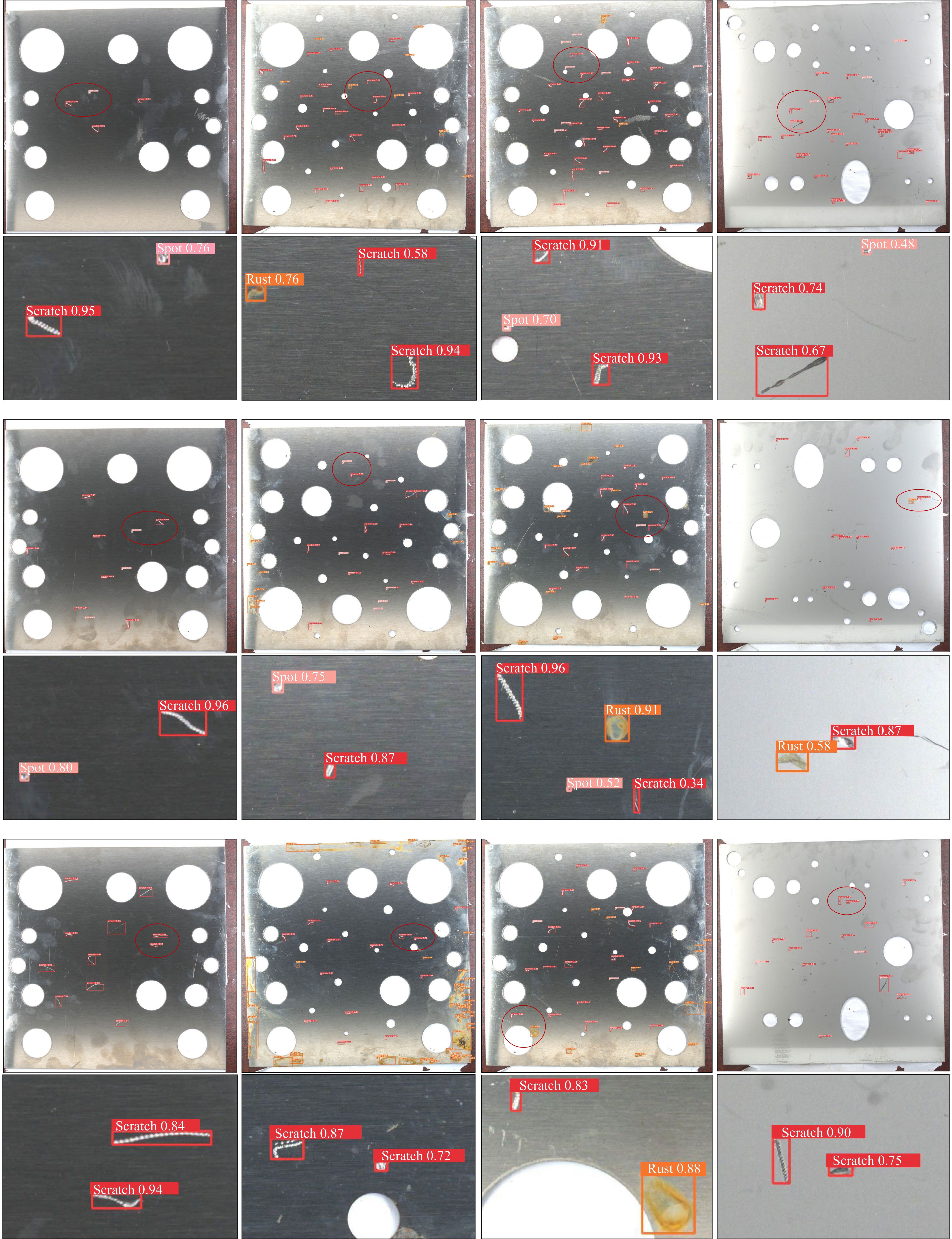
The visualization of the detection results is shown in Fig. 6. Our method is capable of accurately detecting defects, even in cases of complex defects, such as small defects and those with significant variations in size.
For defect segmentation, we implement the CNN-based and Transformer-based methods mentioned in 2.4 using MMSegmentation [57]. Most experimental parameters are kept consistent with the default parameters in MMSegmentation. For image augmentation, we employ the default configurations from MMSegmentation. During training, random flip, photometric distortion are used to augment the data. When using multiple losses, the weight of CrossEntropyLoss and DiceLoss are 1.0 and 3.0 respectively. We use 4 NVIDIA GeForce RTX
| Methods | Loss | Optimizer | Scheduler | Learning rate | Weight decay | Momentum | Batch size | Iterations |
| FCN [40] | CE + Dice | SGD | PolyLR | 0.01 | 0.9 | 4 | 80 000 | |
| UNet [41] | CE + Dice | SGD | PolyLR | 0.01 | 0.9 | 2 | 160 000 | |
| DeepLabv3 [42] | CE + Dice | SGD | PolyLR | 0.01 | 0.9 | 4 | 80 000 | |
| DeepLabv3plus [44] | CE + Dice | SGD | PolyLR | 0.01 | 0.9 | 2 | 160 000 | |
| FastFCN [45] | CE + Dice | SGD | PolyLR | 0.01 | 0.9 | 4 | 80 000 | |
| CGNet [46] | CE + Dice | SGD | PolyLR | 0.01 | 0.9 | 4 | 80 000 | |
| DDRNet [47] | CE + Dice | SGD | PolyLR | 0.01 | 0.9 | 4 | 80 000 | |
| PIDNet [48] | CE + Dice | SGD | PolyLR | 0.01 | 0.9 | 4 | 80 000 | |
| Segmenter [49] | CE + Dice | SGD | PolyLR | 0.001 | 0 | 0.9 | 1 | 320 000 |
| Segformer [50] | CE + Dice | SGD | PolyLR | 0.01 | 0.9 | 4 | 80 000 | |
| MaskFormer [51] | CE + Focal + Dice | AdamW | LinearLR + PolyLR | 6E−05 | 0.01 | 0.9 | 4 | 80 000 |
| Mask2Former [51] | CE + Dice | AdamW | PolyLR | 1E−04 | 0.05 | 0.9 | 2 | 160 000 |
DownLoad:
CSV
The performances of all the CNN-based and Transformer-based methods on our CSDD for defect segmentation are presented in the Table VII. Among all the methods, Unet achieves the best performance, with the mIoU of 54.29%. The CGNet has the lowest model complexity but only reaches the mIoU of 48.20%. Figure ??? shows the visualized segmentation results of the Unet. Most of the defects are accurately segmented. Compared to scratches, spots and rusts are more difficult to segment, highlighting that one of the most challenging aspects lies in identifying small defects and those with significant size variation. This implies that there is still room for improvement in existing methods on our CSDD.
| Method | Scratch | Spot | Rust | Average | Complexity | ||
| IoU% ↑ | mIoU% ↑ | GFLOPs ↓ | |||||
| FCN [40] | 55.63 | 46.80 | 42.54 | 48.32 | 791 | ||
| UNet [41] | 65.73 | 50.64 | 46.49 | 54.29 | 812 | ||
| DeepLabv3 [42] | 53.99 | 45.32 | 41.26 | 46.86 | |||
| DeepLabv3plus [44] | 61.10 | 46.39 | 44.26 | 50.58 | 706 | ||
| FastFCN [45] | 54.79 | 45.77 | 40.52 | 47.03 | 521 | ||
| CGNet [46] | 55.22 | 47.33 | 42.04 | 48.20 | 13.80 | ||
| DDRNet [47] | 46.21 | 35.87 | 36.79 | 39.62 | 71.73 | ||
| PIDNet [48] | 46.70 | 35.99 | 38.21 | 40.30 | 23.76 | ||
| Segmenter [49] | 25.90 | 24.71 | 30.18 | 26.93 | 775 | ||
| SegFormer [50] | 59.13 | 43.67 | 43.89 | 48.90 | 148 | ||
| MaskFormer [51] | 60.81 | 46.07 | 44.05 | 50.31 | − | ||
| Mask2Former [52] | 60.76 | 45.15 | 44.00 | 49.97 | − | ||
DownLoad:
CSV
To further validate the generalizability of our proposed method, we conduct experiments on the NEU-DET and GC10-DET datasets. Similar to the experimental settings employed on the CSDD, the NEU-DET and GC10-DET datasets are subdivided into training, validation, and test sets, with proportions of 64%, 16% and 20%, respectively. The images are also resized to
On the NEU-DET dataset, the standard YOLOv5 achieves the mAP of 62.0%, while our method reaches the mAP of 73.1%, which represents a significant improvement of 11.1%. On the GC10-DET dataset, the standard YOLOv5 exhibits the mAP of 59.5%, while our method achieves the mAP of 64.3%, reflecting an enhancement of 4.8%. These results demonstrate that the global attention mechanism and partial convolution introduced in our method can provide significant performance improvements on both NEU-DET and GC10-DET datasets, further validating the generalizability of our method.
The employment of the GAM and PConv allows our model to capture defect features more precisely and comprehensively, thereby achieving higher defect detection performance across all defect types. Our method achieves the AP of 84.4%, 73.2% and 55.8% for the scratch, spot and rust, respectively. It is noteworthy that, in comparison to the scratch, the spot generally appears in smaller sizes, while the rust tends to have more complex shapes. This indicates that there is still room for improvement in our method for detecting small-sized and complex-shaped defects, which can be a focus for future work.
For the defect detection task, the performance of seven CNN-based methods (Faster RCNN, Cascade R-CNN, SSD, YOLOv5, YOLOv8, YOLOv10 and CenterNet) outperforms that of the best Transformer-based method (Conditional DETR). These results suggest that the perception of local features may be more important. CNNs, through convolutional layers, effectively extract local features, which are crucial for capturing low-level information such as the edges and textures of defects in images. Furthermore, CNNs can effectively maintain the spatial structure of the image, making them well suited for handling spatially localized information.
1) Multimodality: Our CSDD can be expanded into a multimodal dataset. In future work, we can add corresponding textual descriptions for each type of defects, serving as prior knowledge about the defects. How to utilize this prior knowledge to further enhance the model’s defect detection performance is a research topic worthy of exploration.
2) Incomplete labels: In some application scenarios, the process of annotating all defects is very labor-intensive and time-consuming. Consequently, research into achieving higher accuracy in defect detection and segmentation with only a subset of defects annotated is a highly valuable direction of study.
In this work, we construct the casting surface defect dataset (CSDD), which contains
| [1] |
J. Masci, U. Meier, G. Fricout, and J. Schmidhuber, “Multi-scale pyramidal pooling network for generic steel defect classification,” The 2013 International Joint Conference on Neural Networks (IJCNN), pp. 1–8, 2013.
|
| [2] |
R. Ren, T. Hung, and K. C. Tan, “A generic deep-learning-based approach for automated surface inspection,” IEEE transactions on cybernetics, vol. 48, no. 3, pp. 929–940, 2017.
|
| [3] |
V. Natarajan, T.-Y. Hung, S. Vaikundam, and L.-T. Chia, “Convolutional networks for voting-based anomaly classification in metal surface inspection,” 2017 IEEE International Conference on Industrial Technology (ICIT), pp. 986–991, 2017.
|
| [4] |
X. Tao, D. Zhang, W. Ma, X. Liu, and D. Xu, “Automatic metallic surface defect detection and recognition with convolutional neural networks,” Applied Sciences, vol. 8, no. 9, p. 1575, 2018. doi: 10.3390/app8091575
|
| [5] |
T. Wang, Y. Chen, M. Qiao, and H. Snoussi, “A fast and robust convolutional neural network-based defect detection model in product quality control,” The International Journal of Advanced Manufacturing Technology, vol. 94, pp. 3465–3471, 2018. doi: 10.1007/s00170-017-0882-0
|
| [6] |
Y.-J. Cha, W. Choi, G. Suh, S. Mahmoudkhani, and O. Büyüköztürk, “Autonomous structural visual inspection using region-based deep learning for detecting multiple damage types,” Computer-Aided Civil and Infrastructure Engineering, vol. 33, no. 9, pp. 731–747, 2018. doi: 10.1111/mice.12334
|
| [7] |
L. Cui, X. Jiang, M. Xu, W. Li, P. Lv, and B. Zhou, “Sddnet: A fast and accurate network for surface defect detection,” IEEE Transactions on Instrumentation and Measurement, vol. 70, pp. 1–13, 2021.
|
| [8] |
X. Jiang, F. Yan, Y. Lu, K. Wang, S. Guo, T. Zhang, Y. Pang, J. Niu, and M. Xu, “Joint attention-guided feature fusion network for saliency detection of surface defects,” IEEE Transactions on Instrumentation and Measurement, vol. 71, pp. 1–12, 2022.
|
| [9] |
H. Wang, R. Zhang, M. Feng, Y. Liu, and G. Yang, “Global contextbased self-similarity feature augmentation and bidirectional feature fusion for surface defect detection,” IEEE Transactions on Instrumentation and Measurement, vol. 72, pp. 1–12, 2023.
|
| [10] |
H. Zhou, R. Yang, R. Hu, C. Shu, X. Tang, and X. Li, “Etdnet: Efficient transformer-based detection network for surface defect detection,” IEEE Transactions on Instrumentation and Measurement, vol. 72, pp. 1–14, 2023.
|
| [11] |
Y. Li, X. Wang, Z. He, Z. Wang, K. Cheng, S. Ding, Y. Fan, X. Li, Y. Niu, S. Xiao et al, “Industry-oriented detection method of pcba defects using semantic segmentation models,” IEEE/CAA Journal of Automatica Sinica, vol. 11, no. 6, pp. 1438–1446, 2024. doi: 10.1109/JAS.2024.124422
|
| [12] |
Y. Han, L. Wang, Y. Wang, and Z. Geng, “Intelligent small sample defect detection of concrete surface using novel deep learning integrating improved yolov5,” IEEE/CAA Journal of Automatica Sinica, vol. 11, no. 2, pp. 545–547, 2024. doi: 10.1109/JAS.2023.124035
|
| [13] |
K. Song and Y. Yan, “A noise robust method based on completed local binary patterns for hot-rolled steel strip surface defects,” Applied Surface Science, vol. 285, pp. 858–864, 2013. doi: 10.1016/j.apsusc.2013.09.002
|
| [14] |
D. Tabernik, S. Sela, J. Skvarč, and D. Skočaj, “Segmentation-Based Deep-Learning Approach for Surface-Defect Detection,”Journal of Intelligent Manufacturing, May 2019.
|
| [15] |
J. Božič, D. Tabernik, and D. Skočaj, “Mixed supervision for surface-defect detection: from weakly to fully supervised learning,”Computers in Industry, 2021.
|
| [16] |
T. Schlagenhauf and M. Landwehr, “Industrial machine tool component surface defect dataset,” Data in Brief, vol. 39, p. 107643, 2021. doi: 10.1016/j.dib.2021.107643
|
| [17] |
X. Lv, F. Duan, J.-j. Jiang, X. Fu, and L. Gan, “Deep metallic surface defect detection: The new benchmark and detection network,”Sensors, vol. 20, no. 6, 2020.
|
| [18] |
G. Song, K. Song, and Y. Yan, “Saliency detection for strip steel surface defects using multiple constraints and improved texture features,” Optics and Lasers in Engineering, vol. 128, p. 106000, 2020. doi: 10.1016/j.optlaseng.2019.106000
|
| [19] |
i. i. O. Alexey Grishin, BorisV, “Severstal: Steel defect detection,”2019.[Online]. Available: https://kaggle.com/competitions/severstal-steel-defect-detection
|
| [20] |
G. Jocher, “Ultralytics yolov5,”2020.[Online]. Available: https://github.com/ultralytics/yolov5
|
| [21] |
S. Ren, K. He, R. Girshick, and J. Sun, “Faster r-cnn: Towards real-time object detection with region proposal networks,”Advances in neural information processing systems, vol. 28, 2015.
|
| [22] |
Z. Cai and N. Vasconcelos, “Cascade r-cnn: Delving into high quality object detection,”in Proceedings of the IEEE conference on computer vision and pattern recognition, 2018, pp. 6154–6162.
|
| [23] |
W. Liu, D. Anguelov, D. Erhan, C. Szegedy, S. Reed, C.-Y. Fu, and A. C. Berg, “Ssd: Single shot multibox detector,”Computer Vision– ECCV 2016: 14th European Conference, Amsterdam, The Netherlands, October 11–14, 2016, Proceedings, Part I 14, pp. 21–37, 2016.
|
| [24] |
T.-Y. Lin, P. Goyal, R. Girshick, K. He, and P. Dollar, “Focal loss x for dense object detection,” Proceedings of the IEEE international conference on computer vision, pp. 2980–2988, 2017.
|
| [25] |
X. Zhou, D. Wang, and P. Krähenbühl, “Objects as points,”arXiv preprint arXiv: 1904.07850, 2019.
|
| [26] |
Z. Tian, C. Shen, H. Chen, and T. He, “Fcos: Fully convolutional one-stage object detection,” Proceedings of the IEEE/CVF international conference on computer vision, pp. 9627–9636, 2019.
|
| [27] |
X. Zhu, W. Su, L. Lu, B. Li, X. Wang, and J. Dai, “Deformable detr: Deformable transformers for end-to-end object detection,”arXiv preprint arXiv: 2010.04159, 2020.
|
| [28] |
D. Meng, X. Chen, Z. Fan, G. Zeng, H. Li, Y. Yuan, L. Sun, and J. Wang, “Conditional detr for fast training convergence,” Proceedings of the IEEE/CVF International Conference on Computer Vision, pp. 3651–3660, 2021.
|
| [29] |
G. Jocher, A. Chaurasia, and J. Qiu, “Ultralytics yolov8,”2023. [Online]. Available: https://github.com/ultralytics/ultralytics
|
| [30] |
L. L. e. a. Ao Wang, Hui Chen, “Yolov10: Real-time end-to-end object detection,”arXiv preprint arXiv: 2405.14458, 2024.
|
| [31] |
N. Carion, F. Massa, G. Synnaeve, N. Usunier, A. Kirillov, and S. Zagoruyko, “End-to-end object detection with transformers,” European conference on computer vision, pp. 213–229, 2020.
|
| [32] |
J. A. Tsanakas, D. Chrysostomou, P. N. Botsaris, and A. Gasteratos, “Fault diagnosis of photovoltaic modules through image processing and canny edge detection on field thermographic measurements,”International Journal of Sustainable Energy, 2015.
|
| [33] |
X.-c. Yuan, L.-s. Wu, and Q. Peng, “An improved otsu method using the weighted object variance for defect detection,”Applied surface science, 2015.
|
| [34] |
N. Otsu, “A threshold selection method from gray-level histograms,” IEEE Transactions on Systems, Man, and Cybernetics, vol. 9, no. 1, pp. 62–66, 1979. doi: 10.1109/TSMC.1979.4310076
|
| [35] |
W. C. Li and D. M. Tsai, “Automatic saw-mark detection in multicrystalline solar wafer images,”Solar Energy Materials and Solar Cells, 2011.
|
| [36] |
Y. G. Cen, R. Z. Zhao, L. H. Cen, L. H. Cui, Z. J. Miao, and W. Zhe, “Defect inspection for tft-lcd images based on the low-rank matrix reconstruction,”Neurocomputing, 2015.
|
| [37] |
C. Jian, J. Gao, and Y. Ao, “Automatic surface defect detection for mobile phone screen glass based on machine vision,” Applied Soft Computing, vol. 52, pp. 348–358, 2017. doi: 10.1016/j.asoc.2016.10.030
|
| [38] |
N. Zeng, P. Wu, Z. Wang, H. Li, W. Liu, and X. Liu, “A smallsized object detection oriented multi-scale feature fusion approach with application to defect detection,” IEEE Transactions on Instrumentation and Measurement, vol. 71, pp. 1–14, 2022.
|
| [39] |
S. Jain, G. Seth, A. Paruthi, U. Soni, and G. Kumar, “Synthetic data augmentation for surface defect detection and classification using deep learning,” Journal of Intelligent Manufacturing, pp. 1–14, 2022.
|
| [40] |
J. Long, E. Shelhamer, and T. Darrell, “Fully convolutional networks for semantic segmentation,” Proceedings of the IEEE conference on computer vision and pattern recognition, pp. 3431–3440, 2015.
|
| [41] |
O. Ronneberger, P. Fischer, and T. Brox, “U-net: Convolutional networks for biomedical image segmentation,”Medical Image Computing and Computer-Assisted Intervention–MICCAI 2015: 18th International Conference, Munich, Germany, October 5-9, 2015, Proceedings, Part Ⅲ 18, pp. 234–241, 2015.
|
| [42] |
L.-C. Chen, G. Papandreou, F. Schroff, and H. Adam, “Rethinking atrous convolution for semantic image segmentation,”arXiv preprint arXiv: 1706.05587, 2017.
|
| [43] |
L.-C. Chen, G. Papandreou, I. Kokkinos, K. Murphy, and A. L. Yuille, “Deeplab: Semantic image segmentation with deep convolutional nets, atrous convolution, and fully connected crfs,” IEEE transactions on pattern analysis and machine intelligence, vol. 40, no. 4, pp. 834–848, 2017.
|
| [44] |
L.-C. Chen, Y. Zhu, G. Papandreou, F. Schroff, and H. Adam, “Encoderdecoder with atrous separable convolution for semantic image segmentation,” Proceedings of the European conference on computer vision (ECCV), pp. 801–818, 2018.
|
| [45] |
H. Wu, J. Zhang, K. Huang, K. Liang, and Y. Yu, “Fastfcn: Rethinking dilated convolution in the backbone for semantic segmentation,”arXiv preprint arXiv: 1903.11816, 2019.
|
| [46] |
T. Wu, S. Tang, R. Zhang, J. Cao, and Y. Zhang, “Cgnet: A light-weight context guided network for semantic segmentation,” IEEE Transactions on Image Processing, vol. 30, pp. 1169–1179, 2020.
|
| [47] |
H. Pan, Y. Hong, W. Sun, and Y. Jia, “Deep dual-resolution networks for real-time and accurate semantic segmentation of traffic scenes,”IEEE Transactions on Intelligent Transportation Systems, 2022.
|
| [48] |
J. Xu, Z. Xiong, and S. P. Bhattacharyya, “Pidnet: A real-time semantic segmentation network inspired by pid controllers,” Proceedings of the IEEE/CVF conference on computer vision and pattern recognition, pp. 19529–19539, 2023.
|
| [49] |
R. Strudel, R. Garcia, I. Laptev, and C. Schmid, “Segmenter: Transformer for semantic segmentation,” Proceedings of the IEEE/CVF international conference on computer vision, pp. 7262–7272, 2021.
|
| [50] |
E. Xie, W. Wang, Z. Yu, A. Anandkumar, J. M. Alvarez, and P. Luo, “Segformer: Simple and efficient design for semantic segmentation with transformers,” Advances in Neural Information Processing Systems, vol. 34, pp. 12077–12090, 2021.
|
| [51] |
B. Cheng, A. Schwing, and A. Kirillov, “Per-pixel classification is not all you need for semantic segmentation,” Advances in Neural Information Processing Systems, vol. 34, p. 17, 2021.
|
| [52] |
B. Cheng, I. Misra, A. G. Schwing, A. Kirillov, and R. Girdhar, “Masked-attention mask transformer for universal image segmentation,” Proceedings of the IEEE/CVF conference on computer vision and pattern recognition, pp. 1290–1299, 2022.
|
| [53] |
Y. Liu, Z. Shao, and N. Hoffmann, “Global attention mechanism: Retain information to enhance channel-spatial interactions,”arXiv preprint arXiv: 2112.05561, 2021.
|
| [54] |
J. Chen, S.-h. Kao, H. He, W. Zhuo, S. Wen, C.-H. Lee, and S.- H. G. Chan, “Run, don’t walk: Chasing higher flops for faster neural networks,” Proceedings of the IEEE/CVF Conference on Computer Vision and Pattern Recognition, p. 12, 2023.
|
| [55] |
S. Woo, J. Park, J.-Y. Lee, and I. S. Kweon, “Cbam: Convolutional block attention module,” Proceedings of the European conference on computer vision (ECCV), pp. 3–19, 2018.
|
| [56] |
K. Chen, J. Wang, J. Pang, Y. Cao, Y. Xiong, X. Li, S. Sun, W. Feng, Z. Liu, J. Xu, Z. Zhang, D. Cheng, C. Zhu, T. Cheng, Q. Zhao, B. Li, X. Lu, R. Zhu, Y. Wu, J. Dai, J. Wang, J. Shi, W. Ouyang, C. C. Loy, and D. Lin, “MMDetection: Open mmlab detection toolbox and benchmark,”arXiv preprint arXiv: 1906.07155, 2019.
|
| [57] |
M. Contributors, “MMSegmentation: Openmmlab semantic segmentation toolbox and benchmark,”https://github.com/open-mmlab/mmsegmentation, 2020.
|
| [1] | Zhenzhen Luo, Xiaolu Jin, Yong Luo, Qiangqiang Zhou, Xin Luo. Analysis of Students’ Positive Emotion and Smile Intensity Using Sequence-Relative Key-Frame Labeling and Deep-Asymmetric Convolutional Neural Network[J]. IEEE/CAA Journal of Automatica Sinica, 2025, 12(4): 806-820. doi: 10.1109/JAS.2024.125016 |
| [2] | Xiaorui Li, Xiaojuan Ban, Haoran Qiao, Zhaolin Yuan, Hong-Ning Dai, Chao Yao, Yu Guo, Mohammad S. Obaidat, George Q. Huang. Multi-Scale Time Series Segmentation Network Based on Eddy Current Testing for Detecting Surface Metal Defects[J]. IEEE/CAA Journal of Automatica Sinica, 2025, 12(3): 528-538. doi: 10.1109/JAS.2025.125117 |
| [3] | Tao Wang, Qiming Chen, Xun Lang, Lei Xie, Peng Li, Hongye Su. Detection of Oscillations in Process Control Loops From Visual Image Space Using Deep Convolutional Networks[J]. IEEE/CAA Journal of Automatica Sinica, 2024, 11(4): 982-995. doi: 10.1109/JAS.2023.124170 |
| [4] | Cong Pan, Junran Peng, Zhaoxiang Zhang. Depth-Guided Vision Transformer With Normalizing Flows for Monocular 3D Object Detection[J]. IEEE/CAA Journal of Automatica Sinica, 2024, 11(3): 673-689. doi: 10.1109/JAS.2023.123660 |
| [5] | Yin Zhu, Qiuqiang Kong, Junjie Shi, Shilei Liu, Xuzhou Ye, Ju-Chiang Wang, Hongming Shan, Junping Zhang. End-to-End Paired Ambisonic-Binaural Audio Rendering[J]. IEEE/CAA Journal of Automatica Sinica, 2024, 11(2): 502-513. doi: 10.1109/JAS.2023.123969 |
| [6] | Wenqi Ren, Yang Tang, Qiyu Sun, Chaoqiang Zhao, Qing-Long Han. Visual Semantic Segmentation Based on Few/Zero-Shot Learning: An Overview[J]. IEEE/CAA Journal of Automatica Sinica, 2024, 11(5): 1106-1126. doi: 10.1109/JAS.2023.123207 |
| [7] | Kailong Liu, Qiao Peng, Yuhang Liu, Naxin Cui, Chenghui Zhang. Explainable Neural Network for Sensitivity Analysis of Lithium-ion Battery Smart Production[J]. IEEE/CAA Journal of Automatica Sinica, 2024, 11(9): 1944-1953. doi: 10.1109/JAS.2024.124539 |
| [8] | Chi Ma, Dianbiao Dong. Finite-time Prescribed Performance Time-Varying Formation Control for Second-Order Multi-Agent Systems With Non-Strict Feedback Based on a Neural Network Observer[J]. IEEE/CAA Journal of Automatica Sinica, 2024, 11(4): 1039-1050. doi: 10.1109/JAS.2023.123615 |
| [9] | Yongming Han, Lei Wang, Youqing Wang, Zhiqiang Geng. Intelligent Small Sample Defect Detection of Concrete Surface Using Novel Deep Learning Integrating Improved YOLOv5[J]. IEEE/CAA Journal of Automatica Sinica, 2024, 11(2): 545-547. doi: 10.1109/JAS.2023.124035 |
| [10] | Dingxin He, HaoPing Wang, Yang Tian, Yida Guo. A Fractional-Order Ultra-Local Model-Based Adaptive Neural Network Sliding Mode Control of n-DOF Upper-Limb Exoskeleton With Input Deadzone[J]. IEEE/CAA Journal of Automatica Sinica, 2024, 11(3): 760-781. doi: 10.1109/JAS.2023.123882 |
| [11] | Yang Li, Xiao Wang, Zhifan He, Ze Wang, Ke Cheng, Sanchuan Ding, Yijing Fan, Xiaotao Li, Yawen Niu, Shanpeng Xiao, Zhenqi Hao, Bin Gao, Huaqiang Wu. Industry-Oriented Detection Method of PCBA Defects Using Semantic Segmentation Models[J]. IEEE/CAA Journal of Automatica Sinica, 2024, 11(6): 1438-1446. doi: 10.1109/JAS.2024.124422 |
| [12] | Zheyun Qin, Xiankai Lu, Xiushan Nie, Dongfang Liu, Yilong Yin, Wenguan Wang. Coarse-to-Fine Video Instance Segmentation With Factorized Conditional Appearance Flows[J]. IEEE/CAA Journal of Automatica Sinica, 2023, 10(5): 1192-1208. doi: 10.1109/JAS.2023.123456 |
| [13] | Ye Lin, Zhezhuang Xu, Dan Chen, Zhijie Ai, Yang Qiu, Yazhou Yuan. Wood Crack Detection Based on Data-Driven Semantic Segmentation Network[J]. IEEE/CAA Journal of Automatica Sinica, 2023, 10(6): 1510-1512. doi: 10.1109/JAS.2023.123357 |
| [14] | Zhijia Zhao, Jian Zhang, Shouyan Chen, Wei He, Keum-Shik Hong. Neural-Network-Based Adaptive Finite-Time Control for a Two-Degree-of-Freedom Helicopter System With an Event-Triggering Mechanism[J]. IEEE/CAA Journal of Automatica Sinica, 2023, 10(8): 1754-1765. doi: 10.1109/JAS.2023.123453 |
| [15] | Lili Fan, Shen Li, Ying Li, Bai Li, Dongpu Cao, Fei-Yue Wang. Pavement Cracks Coupled With Shadows: A New Shadow-Crack Dataset and A Shadow-Removal-Oriented Crack Detection Approach[J]. IEEE/CAA Journal of Automatica Sinica, 2023, 10(7): 1593-1607. doi: 10.1109/JAS.2023.123447 |
| [16] | Jinhu Lü, Guanghui Wen, Ruqian Lu, Yong Wang, Songmao Zhang. Networked Knowledge and Complex Networks: An Engineering View[J]. IEEE/CAA Journal of Automatica Sinica, 2022, 9(8): 1366-1383. doi: 10.1109/JAS.2022.105737 |
| [17] | Yu Cao, Jian Huang. Neural-Network-Based Nonlinear Model Predictive Tracking Control of a Pneumatic Muscle Actuator-Driven Exoskeleton[J]. IEEE/CAA Journal of Automatica Sinica, 2020, 7(6): 1478-1488. doi: 10.1109/JAS.2020.1003351 |
| [18] | Xiaowei Feng, Xiangyu Kong, Hongguang Ma. Coupled Cross-correlation Neural Network Algorithm for Principal Singular Triplet Extraction of a Cross-covariance Matrix[J]. IEEE/CAA Journal of Automatica Sinica, 2016, 3(2): 147-156. |
| [19] | Xiaoming Sun, Shuzhi Sam Ge. Adaptive Neural Region Tracking Control of Multi-fully Actuated Ocean Surface Vessels[J]. IEEE/CAA Journal of Automatica Sinica, 2014, 1(1): 77-83. |
| [20] | Qiming Zhao, Hao Xu, Sarangapani Jagannathan. Near Optimal Output Feedback Control of Nonlinear Discrete-time Systems Based on Reinforcement Neural Network Learning[J]. IEEE/CAA Journal of Automatica Sinica, 2014, 1(4): 372-384. |
Figures(7) / Tables(7)


K. Mao, P. Wei, Y. Wang, M. Liu, S. Wang, and N. Zheng, “CSDD: A benchmark dataset for casting surface defect detection and segmentation,” IEEE/CAA J. Autom. Sinica, vol. 12, no. 5, pp. 1–13, May 2025.
| Dataset | Objects | Structure | Images | Anno. images | Anno. defects | Color mode | Resolution | Anno. type | Defect types |
| NEU-DET [13] | Steel Strip | 200×200 | Bbox | 6 | |||||
| GC10-DET [17] | Metal | 2048×1000 | Bbox | 10 | |||||
| Severstal [19] | Steel | 18074 | 12568 | 1600×256 | Pixel | 4 | |||
| KolektorSDD [14] | Commutator | 399 | 399 | 56 | 1270×500 | Pixel | 1 | ||
| KolektorSDD2 [15] | Commutator | 394 | √ | 649×241 | Pixel | 1 | |||
| SD-saliency-900 [18] | Steel Strip | 900 | 900 | 200×200 | Pixel | 3 | |||
| BSData [16] | Spindle | √ | 485 | √ | 2816×1016 | Pixel | 1 | ||
| CSDD(Ours) | Casting | √ | √ | 3648×3648 | Pixel | 3 |
DownLoad:
CSV
| Type | Number | Width (Avg) | Height (Avg) |
| Scratch | 71.77 | 39.23 | |
| Spot | 24.40 | 20.83 | |
| Rust | 71.55 | 41.34 |
DownLoad:
CSV
| Methods | Optimizer | Learning rate | Weight decay | Momentum | Augmentation | Loss | Scheduler | Batch size | Epochs |
| Faster R-CNN [21] | SGD | 0.02 | 0.9 | Random flip | L1 loss (bbox) CE loss (cls) | Linear LR | 4 | 48 | |
| Cascade R-CNN [22] | SGD | 0.02 | 0.9 | Random flip | Smooth L1 loss (bbox) CE loss (cls) |
Linear LR | 4 | 48 | |
| SSD [23] | SGD | 0.002 | 0.9 | Random crop Random flip |
Smooth L1 loss (bbox) CE loss (cls) |
Linear LR | 4 | 48 | |
| RetinaNet [24] | SGD | 0.02 | 0.9 | Random flip | L1 loss (bbox) Focal loss (cls) |
Linear LR | 4 | 48 | |
| YOLOv5 [20] | SGD | 0.01 | 0.8 | Mosaic, mixup HSV color-space random flip |
CIoU loss (location) BCE loss (class+object) |
Lambda LR | 4 | 300 | |
| YOLOv8 [29] | SGD | 0.01 | 0.8 | Mosaic, mixup HSV color-space random flip |
CIoU loss (location) BCE loss (class+object) |
Lambda LR | 4 | 300 | |
| YOLOv10 [30] | SGD | 0.01 | 0.8 | Mosaic, mixup HSV color-space random flip |
CIoU loss (location) BCE loss (class+object) |
Lambda LR | 4 | 300 | |
| CenterNet [25] | SGD | 0.01 | 0.9 | Random flip | GIoU loss (bbox) Gaussian focal loss (cls) |
Linear LR | 4 | 48 | |
| FCOS [26] | SGD | 0.01 | 0.9 | Random flip | IoU loss (bbox) CE loss (cls) |
Constant LR MultiStep LR | 4 | 48 | |
| Deformable DETR [27] | AdamW | − | Random flip Random crop Random Choice resize |
L1 loss (bbox), Focal loss (cls), GIoU loss (IoU) | MultiStep LR | 4 | 500 | ||
| Conditional DETR [28] | AdamW | − | Random flip Random crop Random Choice resize |
L1 loss (bbox), Focal loss (cls), GIoU loss (IoU) | MultiStep LR | 4 | 500 |
DownLoad:
CSV
| Method | Scratch | Spot | Rust | Average | Complexity | ||
| AP% ↑ | mAP% ↑ | GFLOPs ↓ | |||||
| Faster R-CNN [21] | 78.4 | 63.5 | 36.0 | 59.3 | 220 | ||
| Cascade R-CNN [22] | 77.8 | 63.5 | 38.0 | 60.0 | 248 | ||
| SSD [23] | 79.8 | 69.4 | 47.2 | 65.5 | 351 | ||
| RetinaNet [24] | 69.9 | 55.6 | 21.6 | 49.0 | 210 | ||
| YOLOv5 [20] | 83.6 | 71.3 | 53.7 | 69.5 | 15.8 | ||
| YOLOv8 [29] | 84.1 | 63.6 | 52.1 | 66.6 | 28.4 | ||
| YOLOv10 [30] | 81.6 | 60.1 | 51.5 | 64.4 | 24.5 | ||
| CenterNet [25] | 77.1 | 55.9 | 32.6 | 55.2 | 201 | ||
| FCOS [26] | 72.6 | 37.1 | 26.6 | 45.4 | 201 | ||
| Deformable DETR [27] | 74.0 | 57.5 | 26.2 | 52.6 | 200 | ||
| Conditional DETR [28] | 75.4 | 58.0 | 25.3 | 52.9 | 102 | ||
| Ours | 84.4 | 73.2 | 55.8 | 71.1 | 16.2 | ||
DownLoad:
CSV
| Combination | mAP↑ | GFLOPs ↓ |
| Base model | 69.5 | 15.8 |
| Base model + GAM | 70.0 | 17.2 |
| Base model + PConv | 70.6 | 14.6 |
| Base model + GAM + PConv | 71.1 | 16.2 |
DownLoad:
CSV
| Methods | Loss | Optimizer | Scheduler | Learning rate | Weight decay | Momentum | Batch size | Iterations |
| FCN [40] | CE + Dice | SGD | PolyLR | 0.01 | 0.9 | 4 | 80 000 | |
| UNet [41] | CE + Dice | SGD | PolyLR | 0.01 | 0.9 | 2 | 160 000 | |
| DeepLabv3 [42] | CE + Dice | SGD | PolyLR | 0.01 | 0.9 | 4 | 80 000 | |
| DeepLabv3plus [44] | CE + Dice | SGD | PolyLR | 0.01 | 0.9 | 2 | 160 000 | |
| FastFCN [45] | CE + Dice | SGD | PolyLR | 0.01 | 0.9 | 4 | 80 000 | |
| CGNet [46] | CE + Dice | SGD | PolyLR | 0.01 | 0.9 | 4 | 80 000 | |
| DDRNet [47] | CE + Dice | SGD | PolyLR | 0.01 | 0.9 | 4 | 80 000 | |
| PIDNet [48] | CE + Dice | SGD | PolyLR | 0.01 | 0.9 | 4 | 80 000 | |
| Segmenter [49] | CE + Dice | SGD | PolyLR | 0.001 | 0 | 0.9 | 1 | 320 000 |
| Segformer [50] | CE + Dice | SGD | PolyLR | 0.01 | 0.9 | 4 | 80 000 | |
| MaskFormer [51] | CE + Focal + Dice | AdamW | LinearLR + PolyLR | 6E−05 | 0.01 | 0.9 | 4 | 80 000 |
| Mask2Former [51] | CE + Dice | AdamW | PolyLR | 1E−04 | 0.05 | 0.9 | 2 | 160 000 |
DownLoad:
CSV
| Method | Scratch | Spot | Rust | Average | Complexity | ||
| IoU% ↑ | mIoU% ↑ | GFLOPs ↓ | |||||
| FCN [40] | 55.63 | 46.80 | 42.54 | 48.32 | 791 | ||
| UNet [41] | 65.73 | 50.64 | 46.49 | 54.29 | 812 | ||
| DeepLabv3 [42] | 53.99 | 45.32 | 41.26 | 46.86 | |||
| DeepLabv3plus [44] | 61.10 | 46.39 | 44.26 | 50.58 | 706 | ||
| FastFCN [45] | 54.79 | 45.77 | 40.52 | 47.03 | 521 | ||
| CGNet [46] | 55.22 | 47.33 | 42.04 | 48.20 | 13.80 | ||
| DDRNet [47] | 46.21 | 35.87 | 36.79 | 39.62 | 71.73 | ||
| PIDNet [48] | 46.70 | 35.99 | 38.21 | 40.30 | 23.76 | ||
| Segmenter [49] | 25.90 | 24.71 | 30.18 | 26.93 | 775 | ||
| SegFormer [50] | 59.13 | 43.67 | 43.89 | 48.90 | 148 | ||
| MaskFormer [51] | 60.81 | 46.07 | 44.05 | 50.31 | − | ||
| Mask2Former [52] | 60.76 | 45.15 | 44.00 | 49.97 | − | ||
DownLoad:
CSV
| Dataset | Objects | Structure | Images | Anno. images | Anno. defects | Color mode | Resolution | Anno. type | Defect types |
| NEU-DET [13] | Steel Strip | 200×200 | Bbox | 6 | |||||
| GC10-DET [17] | Metal | 2048×1000 | Bbox | 10 | |||||
| Severstal [19] | Steel | 18074 | 12568 | 1600×256 | Pixel | 4 | |||
| KolektorSDD [14] | Commutator | 399 | 399 | 56 | 1270×500 | Pixel | 1 | ||
| KolektorSDD2 [15] | Commutator | 394 | √ | 649×241 | Pixel | 1 | |||
| SD-saliency-900 [18] | Steel Strip | 900 | 900 | 200×200 | Pixel | 3 | |||
| BSData [16] | Spindle | √ | 485 | √ | 2816×1016 | Pixel | 1 | ||
| CSDD(Ours) | Casting | √ | √ | 3648×3648 | Pixel | 3 |
| Type | Number | Width (Avg) | Height (Avg) |
| Scratch | 71.77 | 39.23 | |
| Spot | 24.40 | 20.83 | |
| Rust | 71.55 | 41.34 |
| Methods | Optimizer | Learning rate | Weight decay | Momentum | Augmentation | Loss | Scheduler | Batch size | Epochs |
| Faster R-CNN [21] | SGD | 0.02 | 0.9 | Random flip | L1 loss (bbox) CE loss (cls) | Linear LR | 4 | 48 | |
| Cascade R-CNN [22] | SGD | 0.02 | 0.9 | Random flip | Smooth L1 loss (bbox) CE loss (cls) |
Linear LR | 4 | 48 | |
| SSD [23] | SGD | 0.002 | 0.9 | Random crop Random flip |
Smooth L1 loss (bbox) CE loss (cls) |
Linear LR | 4 | 48 | |
| RetinaNet [24] | SGD | 0.02 | 0.9 | Random flip | L1 loss (bbox) Focal loss (cls) |
Linear LR | 4 | 48 | |
| YOLOv5 [20] | SGD | 0.01 | 0.8 | Mosaic, mixup HSV color-space random flip |
CIoU loss (location) BCE loss (class+object) |
Lambda LR | 4 | 300 | |
| YOLOv8 [29] | SGD | 0.01 | 0.8 | Mosaic, mixup HSV color-space random flip |
CIoU loss (location) BCE loss (class+object) |
Lambda LR | 4 | 300 | |
| YOLOv10 [30] | SGD | 0.01 | 0.8 | Mosaic, mixup HSV color-space random flip |
CIoU loss (location) BCE loss (class+object) |
Lambda LR | 4 | 300 | |
| CenterNet [25] | SGD | 0.01 | 0.9 | Random flip | GIoU loss (bbox) Gaussian focal loss (cls) |
Linear LR | 4 | 48 | |
| FCOS [26] | SGD | 0.01 | 0.9 | Random flip | IoU loss (bbox) CE loss (cls) |
Constant LR MultiStep LR | 4 | 48 | |
| Deformable DETR [27] | AdamW | − | Random flip Random crop Random Choice resize |
L1 loss (bbox), Focal loss (cls), GIoU loss (IoU) | MultiStep LR | 4 | 500 | ||
| Conditional DETR [28] | AdamW | − | Random flip Random crop Random Choice resize |
L1 loss (bbox), Focal loss (cls), GIoU loss (IoU) | MultiStep LR | 4 | 500 |
| Method | Scratch | Spot | Rust | Average | Complexity | ||
| AP% ↑ | mAP% ↑ | GFLOPs ↓ | |||||
| Faster R-CNN [21] | 78.4 | 63.5 | 36.0 | 59.3 | 220 | ||
| Cascade R-CNN [22] | 77.8 | 63.5 | 38.0 | 60.0 | 248 | ||
| SSD [23] | 79.8 | 69.4 | 47.2 | 65.5 | 351 | ||
| RetinaNet [24] | 69.9 | 55.6 | 21.6 | 49.0 | 210 | ||
| YOLOv5 [20] | 83.6 | 71.3 | 53.7 | 69.5 | 15.8 | ||
| YOLOv8 [29] | 84.1 | 63.6 | 52.1 | 66.6 | 28.4 | ||
| YOLOv10 [30] | 81.6 | 60.1 | 51.5 | 64.4 | 24.5 | ||
| CenterNet [25] | 77.1 | 55.9 | 32.6 | 55.2 | 201 | ||
| FCOS [26] | 72.6 | 37.1 | 26.6 | 45.4 | 201 | ||
| Deformable DETR [27] | 74.0 | 57.5 | 26.2 | 52.6 | 200 | ||
| Conditional DETR [28] | 75.4 | 58.0 | 25.3 | 52.9 | 102 | ||
| Ours | 84.4 | 73.2 | 55.8 | 71.1 | 16.2 | ||
| Combination | mAP↑ | GFLOPs ↓ |
| Base model | 69.5 | 15.8 |
| Base model + GAM | 70.0 | 17.2 |
| Base model + PConv | 70.6 | 14.6 |
| Base model + GAM + PConv | 71.1 | 16.2 |
| Methods | Loss | Optimizer | Scheduler | Learning rate | Weight decay | Momentum | Batch size | Iterations |
| FCN [40] | CE + Dice | SGD | PolyLR | 0.01 | 0.9 | 4 | 80 000 | |
| UNet [41] | CE + Dice | SGD | PolyLR | 0.01 | 0.9 | 2 | 160 000 | |
| DeepLabv3 [42] | CE + Dice | SGD | PolyLR | 0.01 | 0.9 | 4 | 80 000 | |
| DeepLabv3plus [44] | CE + Dice | SGD | PolyLR | 0.01 | 0.9 | 2 | 160 000 | |
| FastFCN [45] | CE + Dice | SGD | PolyLR | 0.01 | 0.9 | 4 | 80 000 | |
| CGNet [46] | CE + Dice | SGD | PolyLR | 0.01 | 0.9 | 4 | 80 000 | |
| DDRNet [47] | CE + Dice | SGD | PolyLR | 0.01 | 0.9 | 4 | 80 000 | |
| PIDNet [48] | CE + Dice | SGD | PolyLR | 0.01 | 0.9 | 4 | 80 000 | |
| Segmenter [49] | CE + Dice | SGD | PolyLR | 0.001 | 0 | 0.9 | 1 | 320 000 |
| Segformer [50] | CE + Dice | SGD | PolyLR | 0.01 | 0.9 | 4 | 80 000 | |
| MaskFormer [51] | CE + Focal + Dice | AdamW | LinearLR + PolyLR | 6E−05 | 0.01 | 0.9 | 4 | 80 000 |
| Mask2Former [51] | CE + Dice | AdamW | PolyLR | 1E−04 | 0.05 | 0.9 | 2 | 160 000 |
| Method | Scratch | Spot | Rust | Average | Complexity | ||
| IoU% ↑ | mIoU% ↑ | GFLOPs ↓ | |||||
| FCN [40] | 55.63 | 46.80 | 42.54 | 48.32 | 791 | ||
| UNet [41] | 65.73 | 50.64 | 46.49 | 54.29 | 812 | ||
| DeepLabv3 [42] | 53.99 | 45.32 | 41.26 | 46.86 | |||
| DeepLabv3plus [44] | 61.10 | 46.39 | 44.26 | 50.58 | 706 | ||
| FastFCN [45] | 54.79 | 45.77 | 40.52 | 47.03 | 521 | ||
| CGNet [46] | 55.22 | 47.33 | 42.04 | 48.20 | 13.80 | ||
| DDRNet [47] | 46.21 | 35.87 | 36.79 | 39.62 | 71.73 | ||
| PIDNet [48] | 46.70 | 35.99 | 38.21 | 40.30 | 23.76 | ||
| Segmenter [49] | 25.90 | 24.71 | 30.18 | 26.93 | 775 | ||
| SegFormer [50] | 59.13 | 43.67 | 43.89 | 48.90 | 148 | ||
| MaskFormer [51] | 60.81 | 46.07 | 44.05 | 50.31 | − | ||
| Mask2Former [52] | 60.76 | 45.15 | 44.00 | 49.97 | − | ||
 DownLoad:

 DownLoad: