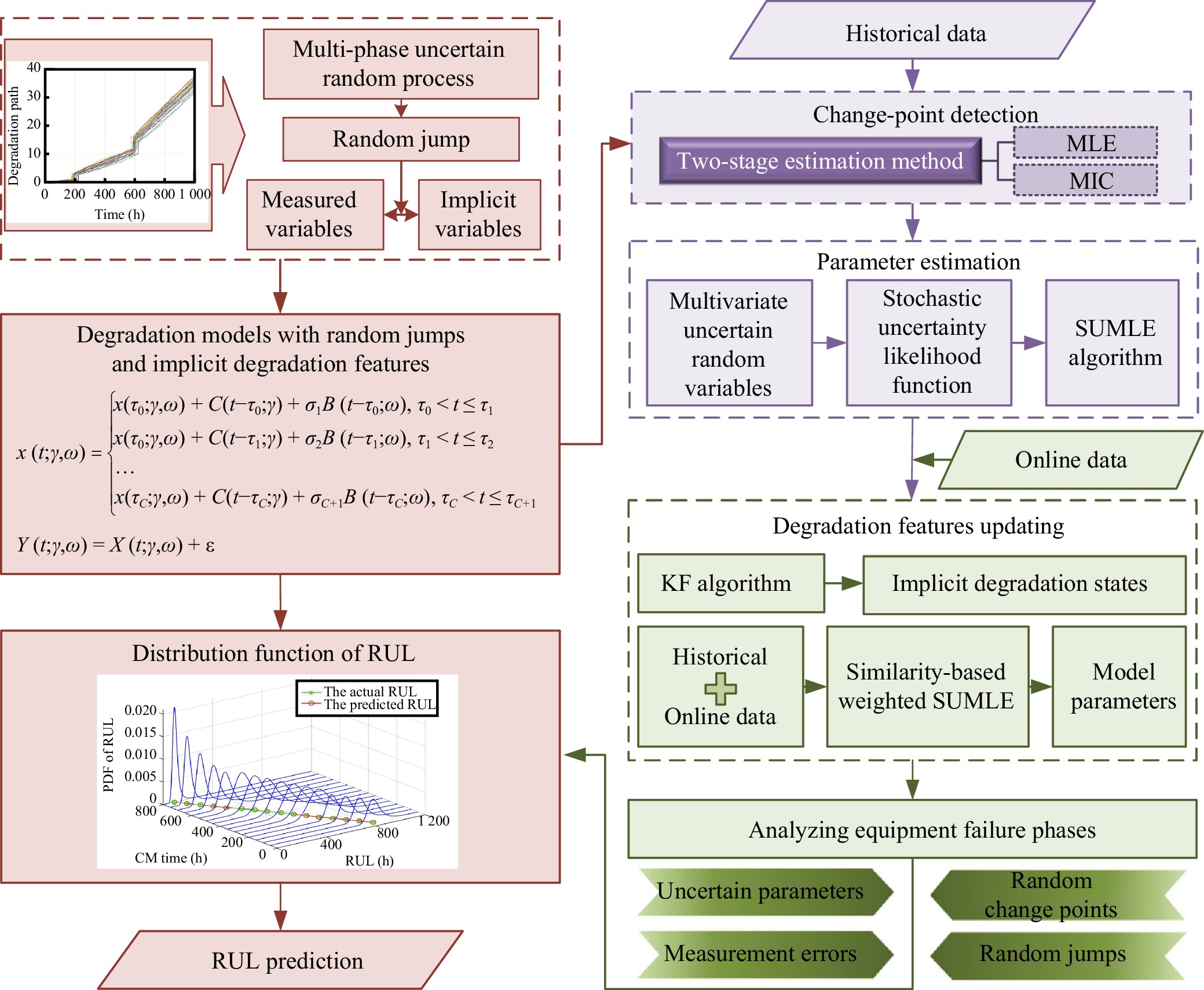
Multi-Phase Degradation Modeling Based on Uncertain Random Process for Remaining Useful Life Prediction Under Triple Uncertainties

I. Introduction

WITH the rapid development of information technology and industry, modern equipment is developing toward large-scale, complicated and intelligent with increasingly high requirements for safety and reliability. As one of the key technologies of new generation equipment, prognosis and health management (PHM) utilizes signal processing and data analysis for detection, assessment, prognostic and management of system health status, according to condition monitoring (CM) data. It plays an essential role in improving the safety, reliability and economy of the equipment [1], [2]. The kernel of PHM is remaining useful life (RUL) prediction based on the existent knowledge, information and data of the degradation process to support the maintenance and management of equipment [3], [4]. Therefore, it is significant for studying accurate and dynamic RUL prediction.

RUL prediction methods are divided into physical model-based methods and data-driven methods [5] according to equipment failure mechanism and performance degradation data. Restricted by product complexity and environmental variability, physical model-based methods are defective in vague failure mechanisms, which are preferred to the research on the bottom essential components [6]. In contrast, data-driven methods achieve RUL prediction based on collected process data, classified as machine learning methods and statistical model-based methods [7]–[9]. The former is more flexible, but it has the disadvantages of low computational efficiency and sensitivity to the quality and quantity of data. The latter is superior in computational efficiency and data requirements, including degenerate trajectory models, stochastic process models, etc. The stochastic process models have significant potential in characterizing dynamic features of the degradation process [10]–[12]. Wiener process is a non-monotonic degenerate process widely employed in RUL prediction and health management because of its excellent mathematical properties.

In practice engineering, the degradation features of some equipment exhibit multi-phase owing to internal factors (e.g., abrupt changes in degradation instrument) or external factors (e.g., dynamic environment, state switching) [13]–[15]. Such complex equipment usually exhibits different degradation patterns throughout its lifecycle. It should be noted that due to abrupt changes in the intrinsic degradation mechanism or the impact of external environmental stresses, the equipment may experience jumps during operation, leading to sudden increases in the degradation states. In recent years, multi-phase degradation model (MPDM) and RUL prediction methods with jumps have received a lot of attention from scholars. Kong et al. [14] proposed a two-phase Wiener process model, which considered an abrupt jump of the change point and gave a reliability assessment method. Gao et al. [15] considered external shocks on the change point in Kong’s model [14] and provided an analytical expression for the life distribution. Further, Wen et al. [16] developed an MPDM based on Wiener process and considered transition probability density function (TPDF) of the degradation states at change points, which calculated RUL based on Monte Carlo method. Liao et al. [17] proposed an MPDM with jumps based on Wiener process, which considered the heterogeneity and derived an expression for RUL under the definition of first hitting time (FHT). Besides, the implicit degradation states of equipment are difficult to obtain due to the interference of external factors such as imperfect measurement environment and measurement noise. Hence, a change-point Wiener process with measurement uncertainty has been investigated in [18]–[20] to adapt to complex equipment characterized by two-phase degradation.

For multi-phase degradation equipment mentioned above, various uncertainties are related to material properties, boundary conditions, and loads in engineering practice. Generally, from the equipment itself, uncertainty can be categorized into aleatory uncertainty and epistemic uncertainty [21]. In addition, measurement uncertainty caused by external measuring devices also exists [22], [23]. Specifically, aleatory uncertainty, also known as objective uncertainty, refers to the randomness characteristics inherent in practice that cannot be eliminated and is typically described by probabilistic models. Representative RUL prediction methods include Wiener process-based methods [24]–[27], hidden Markov-based methods [28], etc. Epistemic uncertainty, also known as subjective uncertainty, is caused by incomplete knowledge and inadequate understanding, which can improve the knowledge of the objective through various scientific practices to reduce epistemic uncertainty. Currently, to account for epistemic uncertainty, a new mathematical theory called uncertainty theory has been introduced for degradation modeling and RUL prediction [29]. The uncertain theory regards the event probability as confidence, which can avoid the confusion of the decision-maker’s combination of frequency probability and subjective probability. It can be used to quantify epistemic uncertainty. In uncertainty theory, an uncertain process can be used to represent degradation trends subject to epistemic uncertainty. The uncertain process in uncertainty theory has been applied to modeling accelerated degradation data and RUL prediction in recent years [30]–[33]. Measurement uncertainty refers to measurement errors caused by imperfect measurement devices, which indicates unavoidable errors in measurement data. Measurement uncertainty is usually quantified by assuming measurement error obeys a normal distribution [20], [22], [23], [34]. However, the problem of RUL prediction for multi-phase degraded equipment under the coexistence of triple uncertainties, i.e., aleatory, epistemic and measurement uncertainties, is neglected in the existing literature.

Although MPDM has received some attention and results, most RUL prediction methods for MPDM are established by stochastic processes. These methods have the following shortcomings: 1) When historical data are limited, there is epistemic uncertainty in the degradation process of equipment due to the lack of sufficient priori knowledge. At this point, it is difficult for stochastic process-based degradation models to accurately fit equipment degradation paths on the basis of a law of large numbers. 2) It is difficult to get implicit degradation states of complex equipment directly because of the limitation of measurement devices or the monitoring environment. Most studies focus on the measurement error of single-phase degraded equipment, while the measurement uncertainty of multi-phase degraded equipment is rarely mentioned. 3) Individual variability among equipment in practical applications is not negligible. It is essential to determine the randomness of change-point times and jumps. Meanwhile, it is challenging to characterize the TPDF of degradation state at the change point under triple uncertainties.

Motivated by these practical issues, this paper proposes a novel MPDM and RUL prediction method with random jumps and implicit degradation features to quantify aleatory, epistemic and measurement uncertainties for a class of complex equipment with multi-phase degradation characteristics. The major contributions are summarized as follows.

$1)$ A novel multi-phase degradation model with random jumps and measurement errors is formulated based on uncertain random processes, where the aleatory uncertainty of degradation trajectory, epistemic uncertainty of degradation parameters and measurement uncertainty of implicit degradation states are expressed.

$2)$ A RUL prediction method with triple uncertainties is proposed considering random jumps and the uncertainties of degradation states at change points. Meanwhile, the analytical expression for RUL is derived based on the concept of FHT under the chance space.

$3)$ An offline training and online updating method that integrates the similarity relationship between historical and online data is proposed to identify model parameters. Two-stage estimation, similarity-based weighted stochastic uncertainty maximum likelihood estimation (SUMLE), and Kalman filtering are used for change point detection, parameter updating, and implicit degradation state updating, respectively.

The rest part of this paper is organized as follows. Section II introduces the problem and MPDM. Section III describes in detail the results of RUL prediction. In Section IV, change point detection, parameter estimation and implicit degradation features updating are provided. Two cases are provided to validate the proposed model in Section V. Finally, conclusions and future works are discussed in Section VI.

II. Problem Description and Multi-Phase Degradation Modeling

As concerned in [13]–[20], [25]–[27], degradation process of complex equipment is characterized by a two-phase or multi-phase affected by internal mutations or external stresses. Specifically, taking rolling bearings as an example, Fig. 1 shows degradation trajectories of four bearings under the same operating conditions. The degradation data show that the bearing 2–3 increases significantly at 122 m, 325 m, 364 m, 428 m, and 523 m, indicating the presence of jumping at the change point. Many researchers have modeled the multi-phase degradation process with jumps at change points and performed RUL prediction [14]–[17]. In addition, four bearings in Fig. 1 differ in the locations of their jumps even though they are operated under the same working conditions and environment, i.e., the jumps of different equipment are random. Meanwhile, collected data are often interfered with by measurement errors in practical applications. If measurement errors are ignored, the accuracy of RUL prediction will decrease. Moreover, aleatory uncertainty induced by inherent fluctuations and epistemic uncertainty generated by limited knowledge are inescapable for complex equipment with small sample data. Therefore, it is essential to investigate MPDM with random jumps and RUL prediction under aleatory, epistemic and measurement uncertainties. Thus, this paper develops a novel multi-phase degradation model based on uncertain random processes (MPDM-URP) considering random jumps to predict RUL under triple uncertainties. The general framework of the proposed method is depicted in Fig. 2.

Figure  1.  Bearing degradation path.

DownLoad: Full-Size Img PowerPoint

Figure  2.  Flowchart of the proposed method

DownLoad: Full-Size Img PowerPoint

For some equipment with random jumps and implicit degradation features, uncertain random processes and measurement equations are combined to fit the degradation path. First, refer to [35], multi-phase uncertain random processes characterize the implicit degradation states for complex equipment. Suppose that $X\left( {t; \gamma, \omega} \right)$ is multiple uncertain random process in chance space $\left( {\Gamma} \times \Omega ,\;{\cal{L}} \times {\mathbb{A}},\;{\cal{M}} \times {{\rm{Pr}}} \right)$ to characterize implicit degradation state at monitoring time t. Assume that there exist C change points and the index positions are ${\boldsymbol{p}} = \left[{p_1},{p_2}, \ldots , {p_C}\right]^\prime$. Let ${p_0} = 0,\;{p_{C + 1}} = M$ and ${p_0} = 0 < {p_1} < {p_2} < \cdots < {p_C} < {p_{C + 1}} = M$, thus the degeneration process is partitioned into $C + 1$ continuity phases,

where $t_{p_c} = \tau_c \left(c = 0,1, \ldots, C\right)$ are the cth change time. Let ${{\boldsymbol{ \tau }}} = {\left[ {\tau _1, \tau _2, \ldots , \tau _C} \right]'}$ and $t_{{p_c}}^ - = \tau _c^ -$ be the left limit. Besides, $X\left( {{\tau _c};\gamma ,\omega } \right) = X\left( {\tau _c^ - ;\gamma ,\omega } \right) + {\delta _c}\left( \omega \right)$ expresses the initial implicit degradation state of the ($c+1$)th phase. ${\boldsymbol{\delta}} = [ {{\delta}_0}\left(\omega\right),{{\delta}_1}\left(\omega\right), \ldots , {{\delta}_{C }}\left(\omega\right) ]'$ is the jump at the change point, where ${\delta_c} \left (\omega \right)$ is a random variable to describe the randomness of the jump which follows a normal distribution ${\delta _c}\left( \omega \right) \sim N( \mu_{\delta _c}, \sigma_{\delta _c}^2 )$. Besides, ${\xi _{c + 1}}\left( \gamma \right) \left( {t - {\tau _c}} \right)$ is the drift term of the $(c+1)$th phase describing the degradation severity, and ${\boldsymbol{\xi }} = [ {\xi _1}\left( \gamma \right), {\xi _2}\left( \gamma \right), \ldots , {\xi _{C + 1}}\left( \gamma \right) ]'$ are drift parameters. $\sigma_{c+1} B\left( t- {\tau _c}; \omega \right)$ is the diffusion term of the $( c+1)$th phase representing the inherent time-varying dynamic characteristics in the degradation process, and ${\boldsymbol{\sigma }} = {\left[ {{\sigma _1},{\sigma _2}, \ldots , {\sigma _{C + 1}}} \right]'}$ are diffusion coefficients.

Remark 1: According to the classification method of uncertainties (i.e., whether uncertainty can be reduced by increasing sample information) [21], let drift term ${\xi _{c + 1}}\left( \gamma \right) \left( {t - {\tau _c}} \right)$ and diffusion term $\sigma_{c+1} B\left( t- {\tau _c}; \omega \right)$ be the uncertain process and stochastic process to express epistemic and aleatory uncertainties, respectively. Specifically, since the degradation paths of each individual of similar equipment present different degradation rates affected by the various operating environment, the degradation degree is uncertain. With the number of similar equipment increasing, the uncertainty of drift could be decreased. Thus $\sigma_{c+1} B\left( t- {\tau _c}; \omega \right)$ should be treated as epistemic uncertainty, expressed by the uncertain process in uncertainty space $\left( {\Gamma} ,{\cal{L}} ,{\cal{M}} \right)$, where the drift parameter ${\xi _{c + 1}}\left( \gamma \right)$ follow the normal uncertainty distribution ${\cal{N}}( {e_{{\xi _{c + 1}}},\sigma _{{\xi _{c + 1}}}} )$. On the other hand, the uncertainty of the diffusion process is invariant although the increase in the number of samples. Therefore, $\sigma_{c+1} B\left( t- {\tau _c}; \omega \right)$ should be treated as the aleatory uncertainty expressed by a stochastic process in probability space $\left( \Omega, {\mathbb{A}}, {{\rm{Pr}}} \right)$, and $\left\{ {B\left( t- {\tau _c}; \omega \right), t - {\tau _c} \ge 0} \right\}$ is a standard Brownian motion (BM), $\sigma_{c+1} B\left( t- {\tau _c}; \omega \right) \sim N( {0,{\sigma_{c+1} ^2}(t- {\tau _c})} )$. Thus, the uncertain random process composed of ${\xi _{c + 1}}\left( \gamma \right) ( t - {\tau _c} )$ and $\sigma_{c+1} B\left( t- {\tau _c}; \omega \right)$ is used to characterize the implicit degradation state of equipment

Furthermore, it is almost impossible to measure the hidden degradation status of equipment accurately. Furthermore, the measurement uncertainty introduced by external monitoring equipment should be considered. This paper refers to [20], [22], [23], [31], assuming that the measurement errors in each degradation stage are random variables to characterize measurement uncertainty. Afterward, incorporating measurement errors into the model shown in (1), let $\left\{ Y\left( {t; \gamma, \omega} \right), t \ge 0 \right\}$ be the measurement process to describe the relationship between the measured values and the implicit degradation states.

where ${\boldsymbol{\varepsilon }} = {\left[ {{\varepsilon _1}\left( \omega \right),{\varepsilon _2}\left( \omega \right), \ldots ,{\varepsilon _{C + 1}}\left( \omega \right)} \right]^\prime }$ is the measurement error based on uncertain random degradation models. Meanwhile, $\varepsilon_c \left( \omega \right)$ is an independent random variable in a probability space $\left( {\Omega ,{\mathbb{A}},{{\rm{Pr}}} } \right)$ and follows normal distribution $\varepsilon_c \left( \omega \right) \sim N( {0,\sigma _{\varepsilon_c} ^2} )$.

Remark 2: By transform parameters $\xi_c \left( \gamma \right), \;{\delta_c}\left( \omega \right)$ and ${{\varepsilon_c }}\left( {{\omega }} \right)$, the proposed models (1) and (2) can include models from the existing literature as a specific case.

$1)$ If ${{\varepsilon_c }}\left( {{\omega }} \right) = 0$ and ${\delta_c}\left( \omega \right) = 0$, the proposed MPDM-URP considering triple uncertainties in this paper will be transformed into an MPDM with aleatory and epistemic uncertainties in [35].

$2)$ If $\xi_c \left( \gamma \right)$ is a random variable and ${\delta _c}\left( \omega \right) = 0$, the proposed MPDM-URP will be simplified as an MPDM [34] under a probability space considering aleatory and measurement uncertainties, which ignores jumps and epistemic uncertainty.

$3)$ If $\xi_c \left( \gamma \right)$ is a random variable and ${{\varepsilon_c }}\left( {{\omega }} \right) = 0$, the proposed MPDM-URP will be transformed into an MPDM based on Wiener process [17], which only concerns aleatory uncertainty.

According to FHT [36], the lifetime of the equipment is defined as the time at which the failure threshold of the monitoring data is reached for the first time. The lifetime described in (1) and (2) is denoted by

where z is the failure threshold.

The degradation measurements data at CM times ${t_0}<{t_1}< \cdots<{t_k}$ are ${{\boldsymbol{Y}}_{{\bf{0:}}{\boldsymbol{k}}}} = \left[ {{y_1},{y_2}, \ldots ,{y_k}} \right]'$ whose corresponding implicit degradation states are ${{\boldsymbol{X}}_{{\bf{0:}}{\boldsymbol{k}}}} = \left[ {{x_1},{x_2}, \ldots ,{x_k}} \right]'$, where ${y_k} = Y\left( {t_k;\gamma ,\omega } \right)$ and ${x_k} = X\left( {t_k;\gamma ,\omega } \right)$. When given CM data ${{\boldsymbol{Y}}}_{{{\bf{0:}}{\boldsymbol{k}}}}$ and failure threshold z, the RUL $L_k$ is

III. RUL Prediction

A RUL Prediction Based on MPDM-URP With Certain Change Points

First, given the change points and corresponding degradation state, the aleatory and measurement uncertainties are considered. Let measurement data of the target equipment during the monitoring time $0$ to $t_k$ be ${{\boldsymbol{Y}}_{{\bf{0:}}{\boldsymbol{k}}}} = \left[ {{y_1},{y_2}, \ldots ,{y_k}} \right]'$. Let ${{\hat x}_{\left. k \right|k}}$ and ${P_{\left. k \right|k}}$ denote the mean and variance of the implicit degradation state ${x_k}$ estimated by ${{\boldsymbol{Y}}_{{\bf{0:}}{\boldsymbol{k}}}}$, i.e. ${x_k} \sim N\left( {{{\hat x}_{\left. k \right|k}},{P_{\left. k \right|k}}} \right)$. Besides, ${{\hat x}_{\left. k \right|k}}$ and ${P_{\left. k \right|k}}$ can be computed by the implicit degradation state updating in Section IV-C. According to (3), the probability density function (PDF) of RUL with change point ${{\boldsymbol{ \tau }}}$ and parameters ${\boldsymbol{\xi }}, \;{\boldsymbol{\delta}}$ is

Then, the RUL for MPDM-URP with certain change points under the chance space will be estimated that combines aleatory, epistemic and measurement uncertainties. It is assumed that ${\xi _{c + 1}}\left( \gamma \right)$ is normal uncertain variable whose uncertainty distribution is ${\Phi _{m + 1}^{ - 1}\left( \alpha \right)} = {{e_{{\xi _{m + 1}}}} + \frac{{\sqrt 3 {\sigma _{{\xi _{m + 1}}}}}}{\pi }\ln \frac{\alpha }{{1 - \alpha }}}$. Combined with the principle of the uncertain variable [29] and the total probability formula, the analytical expression for the RUL with triple uncertainties and certain change-point times can be derived in the following theorem.

Theorem 1: For MPDM-URP with triple uncertainties in (1) and (2), assuming that change-point time $\tau_c$ and corresponding implicit degradation state $x_{\tau_c}$ are given, the PDF of RUL is

where

The proof is given in Appendix A.

B RUL Prediction Based on MPDM-URP With Random Jumps and Random Change Points

Consider the randomness of change-point times and jumps. Unlike multi-phase degradation model without jumps, the lifetime of multi-phase model with jumps is discontinuous at the change point, i.e., ${x_{{\tau _{c}}}} = {x_{\tau _{c}^ - }} + {\delta _{c}}\left( \omega \right)$, where ${x_{\tau _{c}^ - }} = X\left( {\tau _c^ - ;\gamma ,\omega } \right)$. Attentively, if change points do not occur, ${x_{\tau_c^- }}$ should be a variable rather than a fixed value, determined by the degradation model of the cth phase and the change-point time. The jump also has randomness and is a random variable.

Theorem 2: For the proposed models (1) and (2), the TPDF from ${x_{{\tau _c}}}$ to ${x_{{\tau _{c + 1}}}}$ is

where

The proof is given in Appendix B.

Therefore, we can compute ${g_{{\tau _{c + 1}}}}( {{x_{{\tau _{c + 1}}}}} )$ by the following Corollary 1.

Corollary 1: For the proposed MPDM-URP in (1) and (2), the TPDF ${g_{{\tau _{c + 1}}}}( {{x_{{\tau _{c + 1}}}}} )$ with ${{\rm{Pr}}} \left\{ {T > {\tau _{c+1}}} \right\}$ can be calculated using the following equations:

and

where ${{g_{{\tau _1}}}( {{x_{{\tau _1}}}} )}$ can be calculated by making $c = 0$ and $x_{\tau _c} = 0$ of (7).

Finally, considering the randomness of change-point times and jumps, the RUL of MPDM-URP with aleatory, epistemic and measurement uncertainties is obtained.

Theorem 3: For the proposed MPDM-URP in (1) and (2), the PDF of RUL is

where

and ${{g_{{\tau _c}}}\left( {{x_{{\tau _c}}}} \right)}$ can be calculated by Theorem 2 and Corollary 1.

Remark 3: The ${e_{{\xi _c},k}},\; {\sigma _{{\xi _c},k}},\; \sigma _{c + 1,k}^2$ in the Theorem 3 are the updated parameters by real-time monitoring data. Besides, the ${{\hat x}_{\left. k \right|k}}$ and ${{P}_{\left. k \right|k}}$ in the Theorem 3 represents the updated implicit degradation state and variance according to real-time monitoring data of the target equipment, respectively. The update process will be explained in detail in Section IV-C. Specifically, when the latest data is collected for the target equipment, the model parameters and implicit degradation states are updated in real time according to the similarity-based weighted SUMLE (SW-SUMLE) method and Kalman filtering. The RUL adaptive prediction of the equipment can be achieved by inputting the update results into (18).

IV. Parameter Estimation and Degradation State Updating

A Change Point Detection

In this section, an empirical two-stage estimation method [17] is employed to detect jump change points. First, we determine the number and location of change points by modified information criterion (MIC) [17], [37]. Second, the hyperparameters of change-point times and random jumps are estimated by maximum likelihood estimation (MLE), and the hyperparameters of the jumps are determined simultaneously. Attentively, the drift parameters and measurement errors are assumed to be constant in this subsection.

First, set the measurement value increment as $\Delta {Y_1} = {y_1} - {y_0}, \; \Delta {Y_2} = {y_2} - {y_1}, \ldots ,\Delta {Y_m} = {y_m} - {y_{m - 1}}$. The time increment is $\Delta {T_1} = {t_1} - {t_0}, \Delta {T_2} = {t_2} - {t_1}, \ldots , \Delta {T_m} = {t_m} - {t_{m - 1}}$. Thus, the parameter vector is ${\bf{\Xi }} = {\left( {{{\boldsymbol{\xi}} ,{\boldsymbol{\sigma}} , {\boldsymbol{\varepsilon}} , {\boldsymbol{p}}}} \right)'}$. Besides, the measurement value increment vector ${{\bf{\Delta}} {\boldsymbol{Y}}} = {\left[ {\Delta {Y_1}, \Delta {Y_2}, \ldots , \Delta {Y_m}} \right]'}$ follows a multivariate normal distribution and the log-likelihood function is:

where ${{m_{c + 1}}} = {p_{c + 1}} - {p_c}$.

For convenience of calculation, let $\upsilon_{c + 1} \;=\; {\xi _{c\; +\; 1}}\left( \gamma \right)\;+$ ${\varepsilon _{c + 1}}\left(\omega\right)$. When ${\boldsymbol{p}}$ are given, drift parameters and diffusion coefficients can be acquired by maximizing (11).

Substitute (12) into (11), the likelihood function related to ${\boldsymbol{p}}$ can be obtained. Thus,

When the number of change-points C is given, the locations ${{\boldsymbol{p}}}$ are searched by (13). Meanwhile, the jumps at the change points are estimated, i.e., ${\boldsymbol{\delta }} = [ \Delta Y_{{p_1}}, \Delta Y_{{p_2}}, \ldots, \Delta Y_{{p_C}} ]'$ and ${\delta _{c}^i\left( \omega \right)} = \Delta Y_{{p_c}}^i$.

Furthermore, the MIC is utilized to determine the optimal number of change points. First, according to a fixed number of change points $C = 1, 2, \ldots, C_U$ and $C_U$ is the upper bound, search the position of change points by (13), which is denoted by ${\rm M}\left( C \right) = l( {\left. {\hat {\bf{\Xi }}} \right|{{{\bf{\Delta}} {\boldsymbol{Y}}}},C} )$. Second, the modified information criterion calculated by

where $\tilde{C}$ is a constant, and $M \le {M_U}$.

Finally, evaluate ${S_{C - 1,C}} = {\mathop{\rm MIC}\nolimits} \left( {C - 1} \right) - {\mathop{\rm MIC}\nolimits} \left( C \right) + 2\log n$, where ${\chi ^ 2} \left (1 \right)$ describes chi-square distribution. Repeat above steps until ${S_{C, C+1}}<\chi_\alpha^2 \left (1 \right)$ and output the number of change points C at this point.

The second stage is to calculate the hyperparameters. Supposing there exist I sets of CM data for historical equipment, the change-point position and time for the ith equipment are represented as ${{\hat{\boldsymbol{p}}}^{{i}}} = [ {\hat p_1^i,\hat p_2^i, \ldots ,\hat p_C^i} ]'$ and ${{\hat{\boldsymbol{\tau}}}^{{i}}} = {[ {\hat \tau _1^i,\hat \tau _2^i, \ldots ,\hat \tau _C^i} ]'}, \;i = 1,2, \ldots, I$. Thus, the hyperparameters of the change-point times and random jumps can be estimated using the following equation, respectively.

and

B Priori Parameter Estimation

In this section, the parameters of MPDM-URP are estimated by SUMLE. Set unknown parameters of the $(c+1)$th phase as vector ${{{\bf{\Theta}}_{{\boldsymbol{c}}+{\bf{1}}} }} = {[ {e_{{\xi _{c+1}}}},{\sigma _{{\xi _{c+1}}}},{\sigma _{c+1}}, \sigma_{\varepsilon_{c+1}} ]'}$, and the parameters are independent. The historical CM data of the ith equipment is noted as ${Y^i}( {{t_{{p_c} + j}};\gamma ,\omega } ) = y_{{p_c} + j}^i, \; i = 1,2, \ldots, I; j = 1,2, \ldots, {m_{c + 1}}$ and $0 < {p_{c + j}} \le m_c$, where ${p_c} + j$ expresses the jth CM at the $c+1$th phase. Therefore, the measurable degradation state is

where ${\xi _{{c + 1}}} ( \gamma ) \sim {\cal{N}}( {e_{{\xi _{c + 1}}},\;\sigma _{{\xi _{c + 1}}}} ),\;{\sigma _{c + 1}}B( {{t_{{p_c} + j}}-{t_{{p_c} }};\; \omega } )\sim N( 0,$ $\sigma _{c + 1}^2 ( {t_{{p_c} + j}}-{t_{{p_c} }}) ), \varepsilon_{c+1}( \omega )\sim N ( 0, \sigma_{\varepsilon_{c+1}} )$.

According to the MPDM-URP in (2), the measurable degradation state $y_{{p_c} + j}^i$ is an uncertain random variable, so the distribution function of degradation state $y_{{p_c} + j}^i$ is

where $F\left( h \right)$ is the normal distribution under a probability space whose mean is $0$ and variance is ${{\sigma ^2} + \sigma _{{\varepsilon _{c + 1}}}^2 + {\sigma_{\delta _c}^2}}$.

In order to calculate the likelihood function of the parameter vector, the following Definition and Lemma are given.

Definition 1 [38]: Let $\xi_1, \xi_2, \ldots, \xi_n$ be independent identically distributed (iid) samples with uncertainty distribution $F \left( z \left| {\boldsymbol{\theta}} \right. \right)$ where ${\boldsymbol{\theta}}$ is a set of unknown parameters, and let $z_1, z_2, \ldots, z_n$ be observed. Then, the likelihood function is defined by

where $\bigwedge$ is the intersection operational representing the operation of taking the smallest in uncertainty theory.

Lemma 1 [38]: Suppose $\xi_1, \xi_2, \ldots, \xi_n$ are iid samples with uncertainty distribution $F \left( z \left| {\boldsymbol{\theta}} \right. \right)$ where ${\boldsymbol{\theta}}$ is a set of unknown parameters. Given that $z_1, z_2, \ldots, z_n$ are observed, if $F \left( z \left| {\boldsymbol{\theta}} \right. \right)$ is differentiable at $z_1, z_2, \ldots, z_n$, then we have

According to the independent assumption, combined with (18), Definition 1 and Lemma 1, the likelihood function of the parameter vector ${\bf{\Theta}} = \left[{{{\bf{\Theta}}_{{\bf{1}}} }}, {{{\bf{\Theta}}_{{\bf{2}}} }}, \ldots, {{{\bf{\Theta}}_{{\boldsymbol{C}}} }}\right]'$ is

where $\Psi '( { {y_{{p_c} + j}^i} |{e_{{\xi _{c + 1}}}},{\sigma _{{\xi _{c + 1}}}},{\sigma _{c + 1}},{\sigma _{{\varepsilon _{c + 1}}}}} )$ is the derivative of $\Psi ( {y_{{p_c} + j}^i} )$, and ${{{ {\boldsymbol{Y}}}_{{\boldsymbol{c}}+{\bf{1}}}^{\boldsymbol{i}}}} = [{{ y_{p_{c+1}}^i}}, {{ y}_{p_{c+2}}^i}, \ldots, {{y}_{n_{c+1}}^i}]'$.

Furthermore, calculate the maximum likelihood estimate of the unknown parameter ${\bf{\Theta}}$ by maximizing (21).

Therefore, prior parameters can be estimated by gradient descent maximize the logarithmic likelihood function $L\left( {\left. {\bf{\Theta }} \right|{{\boldsymbol{Y}}_{{\boldsymbol{c}}+{\bf{1}}}^{\bf{1}}},{{\boldsymbol{Y}}_{{\boldsymbol{c}}+{\bf{1}}}^{\bf{2}}}, \ldots , {{\boldsymbol{Y}}_{{\boldsymbol{c}}+{\bf{1}}}^{\boldsymbol{I}}}} \right)$ to obtain the optimal solution for the parameters. Thus, the estimated value of the prior parameter is denoted as ${e_{{\xi _{c+1,0}}}},{\sigma _{{\xi _{c+1,0}}}},{\sigma _{c+1,0}}, \sigma_{\varepsilon_{c+1},0}$.

C Implicit Degradation Features Updating

In this section, we combine prior information and online CM data ${{{\boldsymbol{Y}}}_{{\bf{1:}}{\boldsymbol{k}}}}$ to update the implicit degradation features. Since the correlation of posterior estimates between the uncertain parameters and implicit degradation state has negligible influence in practice application, they are generally believed to be independent. Therefore, divide the implicit degradation features updating into two steps. First, the SW-SUMLE method is used to update parameters ${e_{{\xi _{c+1,0}}}},\;{\sigma _{{\xi _{c+1,0}}}},\;{\sigma _{c+1,0}}, \sigma_{\varepsilon_{c+1},0}$. The second step is to update the implicit degradation state $x_k$ using Kalman filtering. Additionally, it should be noted that when change points do not appear, the degradation features of the 1st phase should be updated. If the cth change point occurs, the model parameters for the $(c+1)$th phase need to be updated. Taking the $(c+1)$th phase as an example, we provide the following specific introduction.

1) SW-SUMLE Updates Parameters

By comparing the similarity between historical implicit degradation states and online implicit degradation states, SW-SUMLE is operated to update parameters. The historical and online monitoring data of ${t_0},{t_1}, \ldots ,{t_k}$ are ${{{ {\boldsymbol{Y}}}_{{{{\bf{0:}}{\boldsymbol{k}}}}}^{\boldsymbol{i}}}} = [{{ y_0^i}}, {{ y}_{1}^i}, \ldots, {{y}_{k}^i}]'$ and ${{\boldsymbol{Y}}_{{{0:k}}}} = \left[{{ y}_{0}},{{ y}_{1}},\ldots,{{y}_{k}}\right]'$, respectively. Specifically, by maximizing the weighted likelihood function (23), the hyperparameters of model parameters are continuously updated ${e_{{\xi _{c+1,0}}}},\;{\sigma _{{\xi _{c+1,k}}}},\;{\sigma _{c+1,k}},\; \sigma_{\varepsilon_{c+1},k}$.

where, $w^i$ is a weight factor calculated based on the similarity between the ith historical and target equipment.

The similarity of distance and space between the historical and online equipment at the same CM time are responded to by Euclidean distance and cosine distance to determine the weight factor. The specific calculation steps are shown in Algorithm 1.

2) Kalman Filtering Updates Implicit Degradation States

Using a state space model to represent the degradation process of online equipment at time $t_k \left( \tau_{c}<t_k<\tau_{c+1} \right)$ is as follows:

Algorithm 1 Determine Weight Coefficient $w^i$

Input: Historical data: ${{{ {\boldsymbol{Y}}}_{{{{\bf{0:}}{\boldsymbol{k}}}}}^{\boldsymbol{i}}}}= [{{ y_0^i}}, {{ y}_{1}^i}, \ldots, {{y}_{k}^i}]'$.

　　　Online monitoring data: ${{{{\boldsymbol{Y}}_{{{{\bf{0:}}{\boldsymbol{k}}}}}}}}=\left[{{ y}_{0}},{{ y}_{1}},\ldots,{{ y}_{k}}\right]'$.

　　　Prior parameters: ${e_{{\xi _{c+1,0}}}},{\sigma _{{\xi _{c+1,0}}}},{\sigma _{c+1,0}}, \sigma_{\varepsilon_{c+1},0}$.

Output: Coefficient: $w^i$

1: Calculate the Euclidean and cosine distance of ${\boldsymbol{y}}_{ K}^i = ( {{t_k},{{y}_{ K }^i} })$ and ${\boldsymbol{y}}_{ K} = \left( {{t_k}, {{y}_{ K }} }\right), K=1,2, \ldots, k$.

2: Calculate the average similarity index.

　where $\tilde d_{1,K}^i = \frac{1}{{d_{1,K}^i}}$ is the distance similarity, and $\tilde d_{2,K}^i = \frac{1}{{d_{2,K}^i}}$ is the direction similarity.

3: Standardize indicators $D_1^i$ and $D_2^i$ as follows:

4: Determine weight coefficients

5: Once new monitoring data are detected, repeat Steps 1−4 until the equipment fails.

where $\xi_{c+1,0} \left( \gamma \right)$ has been obtained in Section IV-B. Let $\xi_{c+1,0} \left( \gamma \right) = {e_{{\xi _{c+1},0}}}$, $\Delta {t_k} = t_k - t_{k-1}$, ${v_{k}} = {\sigma_{c+1,k} ^2}[ B\left( {{t_k}}; \omega \right) - B( {{t_{k - 1}}}; \omega ) ]$. $\left\{ {{\nu _{k}}} \right\}$ and $\left\{ {\varepsilon _{c+1,k}} \left( \omega \right) \right\}$ be independent and identically distributed noise sequences, and ${\nu _{k}} \sim N( {0,{\sigma_{c+1,k} ^2}\Delta {t_k}} )$, ${\varepsilon _{c+1,k} \left( \omega \right)} \sim N( {0,\sigma _{\varepsilon_{c+1},k} ^2} )$.

The state space model in (24) is considered as input, and Kalman filtering is operated to estimate the implicit degradation state ${\hat x_{\left. k \right|k}}$ and variance ${P_{\left. k \right|k}}$ from the initial to current time.

Thus, the implicit degradation states and variances can be estimated iteratively by Kalman filtering as follows.

State estimation:

Variance update:

According to the settings in previous section, the initial values are ${\hat x_{\left. 0 \right|0}} = {\mu _{{\delta _c}}},\;{P_{\left. 0 \right|0}} = 0$. The posterior estimate of $x_k$ can be solved by repeating (25) and (26). Therefore, the implicit degradation states of target equipment can be obtained.

V. Case Study

In this section, a numerical example and practical case are operated to expound the significance of the proposed MPDM-URP method and compare the predicted values with some current methods. Specifically, MPDM with aleatory and epistemic uncertainties in [35] and Wiener process-based MPDM with random jumps in [17] are used for comparative verification, respectively. Besides, the mean absolute percentage error (MAPE), cumulative relative accuracy (CRA), and confidence interval (CI), which are commonly employed in RUL prediction, are used to quantify prediction results.

where, let $W\left( {{l_k}} \right) = 1$ mean the identical weigh and $RA_k = 1 -$ $\frac{{\left| {{l_k} - {{\tilde l}_k}} \right|}}{{\tilde l}_k}$.

A Simulation Example

A simulation example with two change points is given to demonstrate the validity of the proposed RUL prediction method. 21 sets of degraded data with time interval $\bigtriangleup t = 2$ are generated by Monte Carlo simulation, of which 20 sets of data are operated as the training set and 1 set of data is operated as the testing level, as shown in Fig. 3. Besides, the simulation parameters are designated as $e_{\xi_1} = 0.004,\; \sigma_{\xi_1} = 0.0005,\; \sigma_1 = 0.02,$ $\mu_{\tau_1} = 100,\; \;\sigma_{\tau_1} = 10,\; \;\mu_{\delta_1} = 2,$ $\sigma_{\delta_1} = 0.05, \;\;\sigma_{\varepsilon_1} = 0.01, e_{\xi_2} = 0.02, \;\sigma_{\xi_2} = 0.005,$ $\sigma_2 = 0.04, \; \mu_{\tau_2} = 300, \;\sigma_{\tau_2} = 10,$ $\mu_{\delta_2} = 4,\;\; \sigma_{\delta_2} = 0.1, \;\;\sigma_{\varepsilon_2} = 0.02,$ $e_{\xi_3} = 0.05, \;\;\sigma_{\xi_3} = 0.01,\;\;\sigma_3 = 0.05, \sigma_{\varepsilon_3} = 0.01$ and the failure threshold is $z = 30$. Thus, data in Fig. 3(b) are operated to verify the proposed MPDM-URP.

Figure  3.  Simulated degradation paths.

DownLoad: Full-Size Img PowerPoint

The change-point detection method in Section IV-A is performed to estimate change-point parameters, and the estimated results are displayed in Table I. Corresponding to [17], [37], set $\tilde{C} = 1$ and $\chi_{0.99}^2 (1) = 6.6349$ with a confidence level of $\alpha = 0.01$. As shown in TABEL I, $S_{2,3} = {\rm MIC}(M = 2)- {\rm MIC}(M = 3)\;+\;2\log(500) \;=\; -0.0562$, and $S_{2,3}\;<\;\chi_{0.99}^2 (1)$. Thus, $C = 2$. Besides, according to (15) and (16), the hyper-parameters of the change-point time and random jumps are calculated showing in Table I.

Table  I.  Results of Change-Point Detection for Simulation

Change-point number	MIC	Change-point locations	Change-point times	$S_{C-1.C}$
0	−15.0839	−	−	−
1	−260.8215	278.5938	557.1876	258.1669
2	−354.6493	102.8193,	205.6386,	106.2569
		304.4457	608.8914
3	−342.1638	97.5116,	195.0232,	−0.0562
		211.0519,	422.1038,
		309.5868	619.1736

 | Show Table

DownLoad: CSV

Besides, the drift parameters, diffusion coefficients and measurement errors of MPDM-URP are computed by SUMLE method illustrated in TABEL II. Furthermore, based on the current monitoring data, the implicit degradation features are synchronously updated by the method described in Section IV-C, where the posterior estimations of the target equipment in the first phase are illustrated in Fig. 4. Due to space limitations, the update processes for the second and third stages are omitted here. With the continuous accumulation of online CM data, the uncertainty gradually decreases, and the model parameters of the equipment tend to be stable.

Table  II.  Results of Parameter Estimation for Simulation

Parameters		$c=1$	$c=2$	$c=3$
$\xi_c\left(\gamma\right)$	$e_{\xi_c}$	0.004 575	0.018 333	0.051 796
	$\sigma_{\xi_c}$	0.000 376	0.004 835	0.010 257
	$\sigma_c$	0.015 682	0.043 036	0.050 639
$\varepsilon_c\left(\omega\right)$	$\sigma_{\varepsilon_c}$	0.009 988	0.023 526	0.009 132
$\delta_c\left(\omega\right)$	$\mu_{\delta_c}$	2.0818	4.0493	−
	$\sigma_{\delta_c}$	0.0557	0.1029	−
$\tau_c$	$\mu_{\tau_c}$	102.8193	304.4457	−
	$\sigma_{\tau_c}$	7.6763	12.1544	−

 | Show Table

DownLoad: CSV

Figure  4.  Implicit degradation feature update for the first phase.

DownLoad: Full-Size Img PowerPoint

RUL estimate of the target equipment at each monitoring point is computed by (10) shown in Fig. 5. It can be observed that the actual and predicted RULs marked with green asterisks and red circles are included in the corresponding PDF. On the other hand, the predicted value of MPDM-URP is proximate to the actual value in the prediction period, indicating that the proposed degradation model considering triple uncertainties can characterize the degradation trend of complex equipment accurately.

Figure  5.  PDF of RUL for the simulation.

DownLoad: Full-Size Img PowerPoint

In addition, MAPE, CRA and CI of MPDM-URP and the methods in [17], [35], are computed to contrast the RUL result quantitatively displaying in Table III and Fig. 6, respectively. We can conclude that the proposed method is superior in dealing with aleatory, epistemic and measurement uncertainties of RUL prediction with random jumps. Compared with the existing methods, the RUL prediction results of MPDM-URP are much close to the actual RUL. Comparatively, [35] focuses on representing aleatory and epistemic uncertainties while ignoring the implicit degradation features and random jumps of equipment. Although [17] expresses aleatory and random jumps, it is a probability-based approach that does not adequately describe epistemic uncertainty under limited data. In addition, measurement uncertainty caused by external devices is ignored.

Table  III.  Comparative Results for Simulation

Method	MPDM-URP	[35]	[17]
MAPE	${\bf{1.3244\%}}$	$2.4875\%$	$5.4724\%$
CRA	0.9868	0.9751	0.9453

 | Show Table

DownLoad: CSV

Figure  6.  CI of RUL prediction of simulation.

DownLoad: Full-Size Img PowerPoint

B Practical Example

In this section, XJTU-SY bearing datasets [39] containing complete run-to-failure data of rolling element bearings are used to illustrate the serviceability of the proposed MPDM-URP in practice. The vibration signals of rolling bearings over their entire life cycle are captured by accelerated life testing to form this dataset. The sampling frequency is 37.5 Hz with a sampling interval of 1 m. The collected horizontal vibration signals are shown in Fig. 7. Additionally, we extract degradation information of bearing using time-domain features. The peak value of the horizontal vibration signal reflects the degradation characteristics of the bearing and perform smoothing to obtain degradation data that characterize the degradation process as shown in Fig. 1. There are inherent fluctuations and individual variability in the various sets of degradation data, reflecting the aleatory and epistemic uncertainties of bearings, as well as measurement uncertainty due to the uncertainty of the signal detection devices. In this dataset, the rapid degradation of Bearings 2−4 in the early stages of operation results in a low degradation reference value. Therefore, this section uses the degradation data of Bearings 2−1, 2−2, 2−3, and 2−5 for experimental verification. Besides, Bearings 2−1, 2−2 and 2−5 are employed as training data, and Bearing 2−3 is operated for RUL prediction. In addition, the failure threshold is set as $z = 30$.

Figure  7.  The horizontal vibration signals of bearings.

DownLoad: Full-Size Img PowerPoint

Similar to the simulation example, we conduct change point detection, model parameter estimation, and implicit degradation feature updates according to the bearing degradation data, whose results are illustrated in Tables IV and V. Besides, the implicit degradation states of Bearing 2−3 is estimated by (25) and (26) displaying in Fig. 8.

Table  IV.  Results of Change-Point Detection for Bearing 2−3

Change-point number	MIC	Change-point times	$S_{C-1.C}$
0	680.1941	−	−
1	−203.6293	278.5938	896.3729
2	−404.5915	115.1384, 317.3909	213.5117
3	−392.1260	115.0171, 317.3927,	0.0840
		363.8011

 | Show Table

DownLoad: CSV

Table  V.  Results of Parameter Estimation for Bearing 2−3

Parameters		$c=1$	$c=2$	$c=3$
$\xi_c\left(\gamma\right)$	$e_{\xi_c}$	−0.003 629	0.007 410	0.155 033
	$\sigma_{\xi_c}$	0.000 144	0.000 587	0.016 040
	$\sigma_c$	0.001 119	0.003 231	0.075 572
$\varepsilon_c\left(\omega\right)$	$\sigma_{\varepsilon_c}$	0.000 127	0.008 799	0.005 809
$\delta_c\left(\omega\right)$	$\mu_{\delta_c}$	2.7583	1.2668	−
	$\sigma_{\delta_c}$	3.6802	1.4279	−
$\tau_c$	$\mu_{\tau_c}$	115.1384	317.3909	−
	$\sigma_{\tau_c}$	158.9204	133.8809	−

 | Show Table

DownLoad: CSV

Figure  8.  Implicit degradation states of Bearing 2−3.

DownLoad: Full-Size Img PowerPoint

According to (10), RUL based on MPDM-URP for Bearing 2−3 is calculated. Fig. 9 shows the prediction results. The blue curves express PDF of RUL for Bearing 2−3 at each CM time, and the green and red lines indicate the actual and predicted RUL of the bearing, respectively. It can be observed that the curve of PDF becomes sharper and narrower with time increasing, which indicates that the uncertainty in the prediction of RUL gradually decreases.

Figure  9.  PDF of RUL for bearing.

DownLoad: Full-Size Img PowerPoint

Besides, RUL prediction results for each CM time can be visualized in Fig. 10. It can be observed that the predicted values of the proposed method become increasingly closer to the actual RUL as time increases. This indicates that the proposed method can provide accurate predictions. To illustrate the superiority of the proposed method, MAPE, CRA and CI are employed to evaluate the prediction performance provided in Table VI and Fig. 10. The results demonstrate that MPDM-URP acquires more accurate results in RUL prediction, which simultaneously accommodates aleatory, epistemic and measurement uncertainties, as well as the uncertainties of degradation states at change points and random jumps. In conclusion, the MPDM-URP and RUL prediction methods proposed in this paper demonstrate high prediction accuracy and specific applicability, which can provide a foundation for maintenance decisions such as equipment ordering and optimal replacement of subsequent equipment.

Figure  10.  CI of RUL prediction of Bearing 2−3.

DownLoad: Full-Size Img PowerPoint

Table  VI.  Comparative Results for Bearing 2−3

Method	MPDM-URP	[35]	[17]
MAPE	${\bf{3.5660\%}}$	$5.5719\%$	$5.9693\%$
CRA	0.9643	0.94428	0.9403

 | Show Table

DownLoad: CSV

VI. Conclusion

This paper concentrates on constructing an MPDM-URP with triple uncertainties and deriving analytic expression for RUL that considers random jumps and implicit degradation features. Thereby, aleatory and epistemic uncertainties of the degradation process at each phase are considered, and the relationship between observed variables and latent variables is analyzed to construct MPDM-URP. Afterward, TPDF of the degradation state at the change point is introduced under the concept of FHT by assuming that the change-point times and the jumps are random variables to describe the heterogeneity. The analytic expression of RUL incorporating triple uncertainties under a chance space is further derived. In addition, model identification methods based on MIC, SUMLE, SW-SUMLE, and Kalman filtering are discussed for off-line estimation of parameters and online updating of implied degradation features. Finally, experiments are conducted to demonstrate the effectiveness of the proposed methods by two case studies. However, the following contents of this paper need to be further investigated.

$1)$ This paper simplifies the estimation of change-point times and jumps, which relies on historical data for offline change point detection. How to adaptively detect change points and perform multi-phase division needs further research.

$2)$ This paper assumes that the degradation stages are independent, while the stages may be interrelated in practice. Analyzing the correlation between each degradation stage is a challenge for future work.

Appendix A. Proof For Theorem 1

Based on (5), consider the parameter ${\xi _{c + 1}}\left( \gamma \right)$ as a normal uncertain variable. The PDF of RUL can be derived by combining the expectation theorem for uncertain variables [29] and the total probability theorem.

For the $(c+1 )$th phase, the PDF is

Since ${{f_{\left. {{L_k}} \right|{\boldsymbol{\tau }}, {\boldsymbol{\xi }}, {\boldsymbol{\delta}}, {{{\boldsymbol{Y}}_{{\bf{0:}}{\boldsymbol{k}}}}}}}\left( {\left. {{l_k}} \right|{\boldsymbol{\tau }}, {\boldsymbol{\xi }}, {\boldsymbol{\delta}}, {{{\boldsymbol{Y}}_{{\bf{0:}}{\boldsymbol{k}}}}}} \right)}$ is concerning $\xi_{c+1} \left( \gamma \right)$ increasing $\left( 0, {{a_{c+1}}} \right)$ and decreasing in $\left( {{a_{c+1}}, 1} \right)$, where

Thus, the PDF of RUL considering triple uncertainties can be given by the following equation:

where

Similarly, the PDFs of RUL for $c = 0,1,\ldots,C$ can be obtained.■

Appendix B. Proof for Theorem 2

The following Lemma is given to prove Theorem 2.

Lemma 2 [40]: If $X\left( t \right) = \xi t + \sigma B\left( t \right)$ expresses BM and ${x_0} = 0$, thus TPDF with a threshold z is

According to Lemma 2, we have

Due to the continuity of time, let ${\tau_1^-} = {\tau_1}$.

For the proposed model, the drift parameters ${\xi _1}\left( \gamma \right)$ and change-point time $\tau_1$ are uncertain variable and random variable, respectively. Besides, ${g_{\tau _1^ - }}( { {{x_{\tau _1^ - }}} |{\xi _1}\left( \gamma \right)} )$ is increasing in $\left( {0,\frac{{{x_{{\tau _{1}}}} }}{{\Delta {\tau _{1}}}}} \right)$ and decreasing in $\left( {{\frac{{{x_{{\tau _{1}}}} }}{{\Delta {\tau _{ 1}}}}},1} \right)$, thus

where

Similarly, TPDF from ${x_{{\tau_c}} }$ to $x_{\tau_{c+1}^-}$ can be obtained as

where

According to ${x_{{\tau _{c + 1}}}} = {x_{\tau _{c + 1}^ - }} + {\delta _c}\left( \omega \right)$, the TPDF is

where $p\left(\delta_{c}\left( \omega \right)\right) = \frac{1}{\sqrt {2\pi {\sigma _{{\delta _{c}}}^2 } }} \exp \left[ - {\frac{\left( {\delta_{c}\left( \omega \right) - {\mu _{{\delta_{c }}}}} \right)^2}{2 {\sigma _{\delta _c} ^2 }} }\right]$.■