

Figure
1.
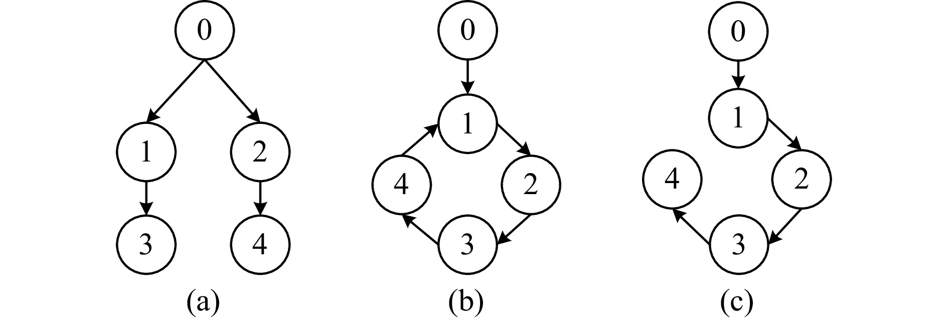
Graphs under Assumptions 3 and/or 4. (a) Typical hierarchical graph; (b) Non-hierarchical graph; (c) Hierarchical graph obtained from graph (b).
 Volume 12
Issue 1
Volume 12
Issue 1
IEEE/CAA Journal of Automatica Sinica
| Citation: | L. Yu and Y. Liu, “Compensation for heterogeneous unknowns and performance-prescribed consensus,” IEEE/CAA J. Autom. Sinica, vol. 12, no. 1, pp. 173–182, Jan. 2025. doi: 10.1109/JAS.2024.124794

|
CONSENSUS, as a primary objective of multi-agent systems (MASs), has attracted extensive attention, and most results specialize in qualitative consensus (without computable boundedness and/or convergence rate) [1]–[8]. Qualitative consensus, however, prevents its wide applications since some vital demands, such as safety and rapidity, could not be guaranteed in the absence of explicit and quantitative performance specifications. As a result, the performance-prescribed consensus emerges, which is a crucial step in pushing consensus forward to real-life applications [9]–[14]. Although a lot of effort has been made on the performance-prescribed consensus, current schemes are relatively restrictive, especially incapable of covering many typical MASs.
The performance-prescribed consensus, for uncertain nonlinear MASs, is much more involved and calls for delicate integrations of compensation/domination and performance guarantee mechanisms. In related works [10]–[12], [14]–[17], prescribed performance control (PPC) and funnel control (FC) are the two most popular schemes. For instance, leaderless and leader-following consensus problems were solved utilizing the PPC scheme in [10] and [11], respectively: The MASs in [10] were subject to quadratic nonlinearities while [11] permitted the systems with parametric uncertainties. However, many MASs may fail to satisfy these requirements since the quadratic or Lipschitz-type conditions generally rule out the heterogeneity of system nonlinearity, and the parameterization form means some known structural information that is critical to the consensus design and performance analysis. By comparison, completely unknown nonlinearities, which require nothing but continuity, encompass a wider range of systems. In this direction, performance-prescribed consensus protocols were proposed in [12], [14]–[17]. Particularly by the FC scheme, [12] achieved leaderless consensus with a prescribed convergence rate under an undirected connected graph and [15] developed a distributed discontinuous controller for the leader-following consensus under a directed graph. Note that [12], [15] achieved consensus in the sense of consensus errors ultimately tending to zero rather than some residual sets as in [14], [16], [17]. Nevertheless, these results (i.e., [12], [14]–[17]) still bear inherent limitations, in particular, requiring the control directions to be known a priori.
The unknown control direction, which could result from some intrinsic uncertainties or serious faults, entails a specialized compensation to recover the desired objective [18]–[20]. While in MASs where multiple unknown control directions are concerned, the compensation mechanisms are harder to construct and the effectiveness is more complicated to achieve, owing to the interconnection between agents in a distributed sense. Currently, the dynamic compensation based on the Nussbaum gain is commonly utilized to cope with unknown control directions, by which, the majority of the related results impose various restrictions on the control coefficients, such as identical signs and/or known magnitude bounds [19], [21]–[24]. More than that, when control directions are unknown, most existing results require uncertainties in the system nonlinearities to be parametric [19], [21]–[23], [25]. This is mainly because sufficient model information is needed for deriving the key lemma (e.g., Lemma 4.1 in [19]) that is the foundation of compensating unknown control directions. When unknown control directions coexist with completely unknown nonlinearities, to the authors’ knowledge, few results have been reported to develop feasible distributed control schemes for consensus. In the context of insufficient system information, if the prescribed performance is further considered, a more powerful control strategy is required which subtly integrates advanced techniques and even develops new ones, in view of the distinct interactions between agents.
The above observations motivate such an issue: In the performance-prescribed context, broaden the range of system classes, while pursuing a precise steady state and a continuous control. To this end, this paper is devoted to performance-prescribed leader-following consensus, for the MASs with completely unknown heterogeneous nonlinearities and nonidentical unknown control coefficients under a directed graph. For the coarse information and prescribed performance, the FC scheme comes as a good choice [12], [18], [26]. Specifically, the first concern raised in the paper is on the MASs with known control directions. Under a directed graph containing a directed spanning tree, a fully distributed protocol is designed, incorporating the funnel gain, prescribed time-varying function and relative states. Therein, the time-varying function is introduced not only to construct the funnel gain but as an indispensable part of the protocol, which substantially enhances the control ability and drives the relative states to zero. Moreover, by invoking a logarithm Lyapunov function candidate, the performance analysis is conducted where the boundedness of the funnel gain plays a key role, especially in guaranteeing the prescribed performance. When the control directions are unknown, a smooth function equipped with varying signs is introduced to combine with the funnel gain, for compensating the unknowns in control coefficients. Remark that in the distributed sense, nonidentical control directions are strongly coupled, causing a failure of the analysis process developed in the known case. This inspires us to seek for the solution from a graphical perspective: a hierarchical graph (defined in Assumption 4) is considered, which is ubiquitous in reality [27]. Owing to the graph hierarchy, the coupling of control directions is essentially simplified. Interestingly, it is found that by choosing proper sub-Lyapunov functions [28], the critical boundedness of the funnel gain can be proved, skillfully following the hierarchical structure [29].
Remarkably, compared with closely related works [15], [16], [19], [21]–[25], [30], the contributions of the paper are highlighted as follows:
1) The considered MASs allow for severe unknowns and heterogeneities, reflected by unknown control coefficients and completely unknown system nonlinearities. Particularly, unknown nonidentical control directions are also involved.
2) Despite the model information available for control design is rather coarse, the consensus is achieved with the prescribed performance and the ultimate convergence of consensus errors (to zero instead of a residual set).
3) The advanced funnel control strategy is leveraged, delicately uniting with the logarithm Lyapunov function or proper graph transformation/simplification, to design a completely relative-state-dependent continuous protocol and analyze the desired performance.
The remainder of the paper is organized as follows. Section II formulates the uncertain nonlinear MASs and the desired objective. Sections III and IV present the design and analysis processes, for the MASs with known and unknown control directions, respectively. In Section V, the theoretical results are applied to simulation examples. Section VI provides some concluding remarks.
Notations: Let R, R+ and R≥t0 represent the sets of real numbers, positive integers and real numbers not less than t0, respectively. Let RN denote the real N-dimensional Euclidean space. Let 0N and 1N denote the N-dimensional column vectors with all entries being 0 and 1, respectively. Let “⊗” denote the standard Kronecker product.
Consider the MASs composed of N followers and one leader (labeled by 0). The dynamics of ith follower, i=1,…,N, is described as
| ˙xi=giui+fi(t,xi) | (1) |
where xi∈R and ui∈R are the system state and the control input, respectively; gi is called the control coefficient which is an unknown nonzero constant whose sign acts as the control direction; fi:R≥t0×R→R is the unknown system nonlinearity which is continuous and locally Lipschitz in its first and second arguments, respectively.
Moreover, the leader x0(t) is a continuously differentiable time-varying signal which is independent of the followers’ information and is only known to a fraction of followers.
With respect to the agent dynamics, two assumptions are imposed on system nonlinearities and the leader, respectively.
Assumption 1: The system nonlinearities fi(t,xi)’s are locally bounded in xi on R, uniform in t on R≥t0; that is, |fi(t,xi)|<+∞ on each bounded set of xi.
Assumption 2: There exists an unknown positive constant M such that
| supt≥t0(|x0(t)|+|˙x0(t)|)≤M. |
In Assumption 1, no prior knowledge of system nonlinearities fi(⋅)’s is imposed, apart from the severe effect of the time variation on them being ruled out. In comparison with the Lipschitz-type or linearly parameterized conditions required in [4], [5], Assumption 1 is milder and provides the protocol design with less information, which naturally gives rise to underlying obstacles for the consensus. In addition, the vanishing property of nonlinearities (i.e., ˉf(0)=0 in [18]) is no longer necessary.
Moreover, differently from the leaders in [5], [23], Assumption 2 indicates that the exact dynamics of the leader are not necessarily known. Only the boundedness of the leader itself and that of its first derivative are required, for guaranteeing the existence of solutions of the closed-loop system.
In this paper, N followers exchange their information via the communication topology modeled by a directed graph G=(V,E), with V={1,2,…,N} and E⊆V×V, respectively denoting the sets of nodes and edges. If (j,i)∈E, then j is called a neighbor of i. Matrix A=[aij]N×N, which satisfies that aij=1, if (j,i)∈E and aij=0, if (j,i)∉E, is the adjacency matrix. In particular, it is assumed aii=0. The associated Laplacian matrix L=[Lij]N×N meets Lij=−aij, for any i≠j and Lii=∑j≠iaij. Furthermore, the augmented graph ˉG=(ˉE,ˉV) with ˉV={0,1,…,N} and ˉE=E∪{(0,i):bi=1}⊆ˉV×ˉV, characterizes the communications among all N+1 agents. Therein, bi=1 means the leader transmits its information to the ith follower and bi=0 otherwise.
Over a directed communication graph ˉG, the control objective of the paper is to achieve the performance-prescribed leader-following consensus, for the MASs composed of N followers described as (1) and one leader x0(t). More specifically, design a fully distributed relative-state-dependent protocol such that
1) For any initial value x(t0)=[x1(t0),…,xN(t0)]∈RN, all the closed-loop system signals are bounded on [t0,+∞);
2) The relative states ξi=∑Nj=1aij(xi−xj)+bi(xi−x0),i=1,…,N, evolve within prescribed performance boundary 1/ϕ(t) and ultimately converge to zero;
where the prescribed time-varying function ϕ(t) satisfies the following three properties which are highly motivated by [18]:
a) ϕ(t) is continuously differentiable on [t0,+∞);
b) ˙ϕ(t)≤c(1+ϕ(t)) with c being a positive constant;
c) ϕ(t0)=0 and ϕ(t)>0, for any t>t0, and furthermore limt→+∞ϕ(t)=+∞.
Remark that there are many typical functions satisfying these three properties, some of them being ϕ(t)=c1(t−t0)c2 and ϕ(t)=c1(ec2t−ec2t0), for any prescribed positive constants c1 and c2. As in the later proof of main theorems, ϕ(t0)=0 plays a key role in relaxing the initial values of system states to be taken in a global sense, and meanwhile the property limt→+∞ϕ(t)=+∞ is rather helpful in enforcing the consensus errors to zero.
In the next two sections, the desired consensus is pursued for followers with known and unknown control directions, respectively. It should be pointed out that although the adopted FC scheme is largely inspired by the single-agent system control, one needs consider the effect of the information interaction among multiple agents in the corresponding performance analysis. We also would like to show in the later development that although both of these two cases resort to FC schemes, quite different analysis processes for the performance-prescribed consensus are required, especially in terms of the structure imposed on the communication graph and the selection of Lyapunov function candidates.
In the section, performance-prescribed leader-following consensus is considered for MASs with known control directions. Without loss of generality, we assume gi>0,i=1,…,N. In addition, the communication topology is modeled by graph ˉG satisfying the following assumption.
Assumption 3: The graph ˉG contains a directed spanning tree with the leader being the root.
In what follows, a useful lemma which can be found in [31], [32] is given.
Lemma 1: If a graph contains a directed spanning tree where the leader is the root, then the following statements hold:
1) The Laplacian matrix associated with graph ˉG can be partitioned as [00TNL2L1], where L1=L+B is a nonsingular M-matrix and B=diag{b1,…,bN};
2) There is a positive diagonal matrix Θ=diag{θ1,…,θN} such that ΘL1+LT1Θ>0.
For each follower with the known control direction, we design a fully distributed protocol based on the relative states
| ui=−ϕ(t)κi(t,ξi)ξi,i=1,…,N | (2) |
where κi(t,ξi)=11−(ϕ(t)ξi)2 is referred to as the funnel gain. Throughout the paper, we will denote κi(t,ξi) for brevity by κi or κi(t) if there is no confusion.
Remark 1: One can see from (2) that the prescribed time-varying function ϕ(t) arises twice: one is in the funnel gain for ensuring the desired performance and the other one directly acts as a part of (2). The former is in line with the FC scheme while the latter helps to remove the requirement for the vanishing property of the system nonlinearities (a critical requirement in [18] to achieve stabilization), though limt→+∞ϕ(t)=+∞ (being critical to enhancing the control ability for driving consensus errors to zero). More specifically, in the later performance analysis (see the proof of Proposition 1), the introduction of the latter ϕ(t) makes (8) still possess one ϕ(t), after forming ϕ2(t)ξ2i. This facilitates extracting one ϕ(t) to avoid the possible unboundedness caused by ϕ(t)|f(t,x)| in (12). Furthermore, the boundedness of ui is guaranteed, as the product term ϕ(t)ξi can elaborately match with the design of κi whose boundedness implies ϕ(t)|ξi|<1.
Define the consensus errors ei=xi−x0,i=1,…,N. With (2), we obtain the error dynamics which can be written in a compact form
| ˙e=−ϕ(t)KGξ+F(t,x)−1N⊗˙x0 | (3) |
where e=[e1,…,eN]T, K=diag{κ1,…,κN}, G=diag{g1,…,gN}, ξ=[ξ1,…,ξN]T, x=[x1,…,xN]T and F(t,x)=[f1(t,x1),…,fN(t,xN)]T.
For the closed-loop system, we first discuss the existence and uniqueness of the solution. Noting the definitions of ξi and ei, one can easily obtain ξ=L1e, by which and the fact L1 being nonsingular M-matrix (according to Assumption 3 and Lemma 1), we define the set
| Ω={(t,e)∈R≥t0×RN|ϕ(t)|ξi|<1,i=1,…,N}. |
First, from the design of the funnel gain, it follows that κ(t)=[κ1(t),…,κN(t)]T is smooth on Ω. Moreover, by the local Lipschitzness in xi and the continuity in t of fi(⋅), and the continuous differentiability of x0(t), we arrive at the fact that the right-hand side of (3) is Lipschitz continuous in e and continuous in t on Ω. Then, owing to ϕ(t0)=0, there is (t0,e(t0))∈Ω, for any initial value e(t0)∈RN. With these in hand, by Theorem 3.1 on page 18 in [33], the closed-loop system has a unique solution (t,e(t))∈Ω on a small interval [0,ts), and furthermore, according to Theorem 2.1 on Page 17 in [33], the solution can be extended to the maximal existence interval [t0,tf) with t0<tf≤+∞.
The following proposition characterizes the dynamic behavior of the relative state vector ξ via a logarithm Lyapunov function candidate. It will be useful in the later proof of Theorem 1 to analyze the consensus. The proof of the proposition is somewhat involved and hence is deferred for better compactness.
Proposition 1: Suppose ξi(t), i=1,…,N, are bounded on [t0,tf). Let V(t,ξ)=∑Ni=112giθilog11−(ϕ(t)ξi)2 with gi and θi being defined in (1) and Lemma 1, respectively. Then, there is a small positive constant δ such that the time derivative of V(⋅) satisfies the following inequality:
| ˙V<ϕ(t)(−δV+¯M) | (4) |
where ¯M is an unknown positive constant.
With Proposition 1 in hand, we next summarize the results which involve followers represented by (1) with known control directions.
Theorem 1: Consider the uncertain nonlinear MASs composed by (1) (with gi>0) and x0(t), under Assumptions 1−3. The fully distributed relative-state-dependent protocol (2) guarantees that, for any initial value x(t0)∈RN, all the closed-loop system signals are bounded on [t0,+∞), and moreover, the relative states evolve within the prescribed boundary formed by 1/ϕ(t) and ultimately converge to zero.
Proof: Due to ϕ(t0)=0, for any ei(t0)∈R, it is straightforward to derive ϕ(t0)|ξi(t0)|<1, i=1,…,N. This implies that a unique solution exists on the maximal existence interval [t0,tf), for any initial value. Then, one can readily obtain that for any t∈[t0,tf), there are
| ϕ(t)|ξi|<1,i=1,…,N. | (5) |
We would like to first show the boundedness of ξi’s and xi’s on [t0,tf). Noting that ϕ(t)>0 for any t>t0 and limt→+∞ϕ(t)=+∞, by the continuity of the closed-loop system, there exist a positive constant ϵ and a time instant t′0∈[t0,tf) such that ϕ(t)>ϵ for any t∈[t′0,tf). Then, from (5), it follows that |ξi(t)|<1/ϕ(t)<1/ϵ<+∞, for any t∈[t′0,tf); namely, we deduce that ξi(t) is bounded on [t0,tf). Noting ξ=L1e and the nonsingular M-matrix L1, we conclude that ei’s are also bounded on [t0,tf). Then, from Assumption 2, one can readily obtain the boundedness of xi’s.
Keeping the boundedness of ξi’s in mind, we next prove the boundedness of κi(t) on [t0,tf) and tf=+∞, as well as the prescribed performance. Invoking Proposition 1, by (4), we can deduce that when V(t)>ˉM/δ, there is ˙V<0. This implies that
| V(t)<max{V(t0),ˉMδ}<+∞,∀t∈[t0,tf) |
which, together with the definition of V(t) in Proposition 1, directly yields the boundedness of κi(t) on [t0,tf), for any i=1,…,N.
Moreover, from the boundedness of ξi and κi, noting (2), we arrive at ui is bounded on [t0,tf) and hence there is no finite escape time, i.e., tf=+∞. Furthermore, since (5) holds for any t≥t0, and noting limt→+∞ϕ(t)=+∞, we can conclude that ξi,i=1,…,N, converge to zero within prescribed performance boundary 1/ϕ(t).
Proof of Proposition 1: Take the time derivative of V(t,ξ). Then, by noting κi=1/(1−(ϕ(t)ξi)2) in (2), one can readily obtain
| ˙V=N∑i=112giθi(1−(ϕ(t)ξi)2)dκi(t)dt=N∑i=1giθiκiϕ(t)˙ϕ(t)ξ2i+N∑i=1giθiκiϕ2(t)ξi˙ξi. | (6) |
Denote the two terms on the right-hand side of (6) by ① and ②, respectively. Noting ˙ϕ(t)≤c(1+ϕ(t)) and ϕ(t)|ξi|<1 for any t∈[t0,tf), by completing the square, we have
| ①<ϕ(t)N∑i=1cgiθiκi(ξ2i+|ξi|)<ϕ(t)(N∑i=1(12γκ2i+γ2(cgiθi(ξ2i+|ξi|))2)) |
with γ being a positive constant determined later.
Then, keeping the boundedness of ξi in mind, we can readily obtain
| ①<ϕ(t)(N∑i=112γκ2i+M1) | (7) |
where M1 is an unknown positive constant.
By ξ=L1x, rewrite ②=ϕ2(t)ξTGKΘL1˙e in a compact form, and invoking (3), we arrive at
| ②=−ϕ3(t)ξTGKΘL1KGξ+ϕ2(t)ξTGKΘL1×(F(t,x)−1N⊗˙x0). |
Denote ΘL1+LT1Θ by ˉΘ, and then from Lemma 1, it follows that:
| −ϕ3(t)ξTGKΘL1KGξ=−ϕ3(t)ξTGKˉΘ2KGξ<−12ϕ(t)λmin(ˉΘ)N∑i=1g2iκ2iϕ2(t)ξ2i. | (8) |
Noting the definition of κi(t)>0, we have ϕ2(t)ξ2i=1− κ−1i, which, together with 12λmin(ˉΘ)∑Ni=1g2iκi≤∑Ni=112γκ2i+ ∑Ni=1γ8(λmin(ˉΘ)g2i)2 (by completing the square) and (8), directly implies
| −ϕ3(t)ξTGKΘL1KGξ<ϕ(t)(N∑i=1(2γ−λmin(ˉΘ)2g2i)κ2i+M2) | (9) |
where M2=∑Ni=1γ8(λmin(ˉΘ)g2i)2 is an unknown positive constant.
Let us proceed the estimation for the second term of ②. Noting ϕ2(t)ξ2i<1 and κi>1, we obtain
| ϕ(t)‖ | (10) |
Moreover, observing \xi=\mathcal{L}_1 e and the definition of e_i , we know that under Assumption 2, the boundedness of \xi_i implies that of x_i . This, together with the continuity of the system nonlinearity, directly guarantees the boundedness of f_i(t,x_i) on [t_0,t_f) . Then, it follows that:
| \|F-{\bf{1}}_N\otimes\dot x_0\|\leq \sqrt{(|f_1|+M)^2+\cdots+(|f_N|+M)^2}\leq M_f | (11) |
with M_f being an unknown positive constant.
Keeping these in mind, by the method of completing the square, it is not hard to obtain that there is an unknown positive constant M_3 such that
| \begin{split} &\phi^2\xi^{{{{{T}}}}}GK\Theta\mathcal{L}_1\left(F(t,x)-{\bf{1}}_N\otimes\dot x_0\right)\\ &\qquad<\phi(t)\sum\limits_{i=1}^{N}\max\limits_{l=1,\ldots,N}\{g_l\theta_l\} \lambda_{\rm{max}}(\mathcal{L}_1)M_f \kappa_i\\ &\qquad<\phi(t)\left(\sum\limits_{i=1}^{N}\frac{2}{\gamma} \kappa^2_i+M_3\right)\end{split} | (12) |
where the first inequality follows by (10) and (11), as well as \|\mathcal{L}_1\|=\lambda_{\rm{max}}(\mathcal{L}_1) , \|\Theta\|=\max_{i=1,\ldots,N}\{\theta_i\} and \|G\|= \max_{i=1,\ldots,N}\{g_i\} . Then, combining (12) with (9), we arrive at
| {\text{②}}<\phi(t)\left(\sum\limits_{i=1}^{N}\left(\frac{1}{\gamma} -\frac{\lambda_{\rm{min}}(\bar\Theta)}{2}g^2_i\right)\kappa^2_i+M_2+M_3\right). | (13) |
Substituting (7) and (13) into (6), one can readily yield
| \dot V<\phi(t)\left(\sum\limits_{i=1}^{N}\left(\frac{3}{2\gamma} -\frac{\lambda_{\rm{min}}(\bar\Theta)}{2}g^2_i\right)\kappa^2_i+\sum\limits_{l=1}^{3}M_l\right). |
Then, taking a sufficiently large \gamma>\frac{3}{\lambda_{\rm{min}}(\bar\Theta)\underline g^2} with \underline g= \min_{i=1,\ldots,N}\{g_i\} , there is a small positive constant \delta immediately such that (4) holds with \bar M=\sum_{l=1}^{3}M_l , owing to \kappa^2_i> \kappa_i>\log \kappa_i (by \kappa_i>1 from its definition).
Remark 2: We would like to elaborate on the necessity of selecting the Lyapunov function candidate in Proposition 1. Intuitively, there are two notable features of the selected V(\cdot) : 1) The “integrated form” reflected by \sum_{i=1}^{N} ; 2) The introduction of logarithm function. Concerning the first feature, with the integrated form of V(\cdot) , the nonsingular \mathcal{M} -matrix \mathcal{L}_1 is utilized to express the correlation of neighboring agents, which essentially avoids the explicit coupling of funnel gains by borrowing some matrix properties. As for the second feature, one can see from (6) and the treatment of ② that the introduction of the logarithm function (especially the characteristics of its derivative) skillfully forms the term -\xi^{{{{{T}}}}}GK\Theta\mathcal{L}_1KG\xi . This is critical to provide the negative term via ensuring (8) for the Lyapunov analysis.
As far as the consensus for MASs with unknown control directions is concerned, most results have imposed different restrictions on the control coefficients, such as identical signs and/or magnitudes with known bounds. More than that, few results, to the authors’ knowledge, permit the coexistence of unknown control directions and prescribed performance requirements, in the context of leader-following consensus. This section is devoted to relaxing the restrictions on control coefficients (involving both the signs and magnitudes) while pursuing asymptotic leader-following consensus with the prescribed performance.
Note that via existing algorithms of graph decomposition [22] or neighbor selection [34], the communication graph under Assumption 3 can be simplified to the one which satisfies:
Assumption 4: The graph \mathcal{\bar G} is connected and has a hierarchical structure, that is, a_{ij} satisfies, for any i,j\in\mathcal{V} , a_{ij}=1 , if (j,i)\in \mathcal{E} and i>j ; a_{ij}=0 otherwise.
Remarkably, the hierarchical graph under Assumption 4 indicates that each agent (except the leader) can only receive the information from its higher levels/hierarchies, requiring fewer links than connected graphs under Assumption 3. For instance, Figs. 1(a) and 1(c) are two typical hierarchical graphs. Particularly, by the graph decomposition, Fig. 1(c) can be obtained from Fig. 1(b) which satisfies Assumption 3. More than that, the graph under Assumption 4 is ubiquitous in real life, such as the status assignment of social animals and large-scale power systems (please refer to [35] for more examples and details).
Then, for the ith follower, i=1,\ldots,N , with unknown control directions, we design the following protocol:
| \left\{\begin{aligned} &u_i=\phi(t)\mathcal{N}(\kappa_i(t,\xi_i))\xi_i \\ &\kappa_i(t,\xi_i)=\frac{1}{1-\left(\phi(t)\xi_i\right)^2} \end{aligned} \right. | (14) |
where \xi_i is defined with new a_{ij} as in Assumption 4, and \mathcal{N}(\cdot) is a smooth function satisfying
| \left\{ \begin{aligned} \lim&\sup\limits_{v\to+\infty}\mathcal{N}(v)=+\infty\\ \lim&\inf\limits_{v\to+\infty}\mathcal{N}(v)=-\infty \end{aligned}\right. | (15) |
which is chosen as \mathcal{N}(v)=v\cos(\pi v) in the paper, inspired by [18].
Remark 3: As is well known, the classical Nussbaum functions \mathcal{M}(\cdot) proposed for compensating the unknown control directions are required to satisfy the following properties:
| \left\{\begin{aligned} \lim&\sup_{l\to+\infty}\frac{1}{l}\int_{0}^{l}\mathcal{M}(v){\rm{d}} v=+\infty\\ \lim&\inf_{l\to+\infty}\frac{1}{l}\int_{0}^{l}\mathcal{M}(v){\rm{d}} v=-\infty. \end{aligned}\right. | (16) |
However, as in related works [19], [21], when being used in the protocol design for consensus, Nussbaum functions satisfying (16) need to be specially constructed for dealing with the coupling of multiple control directions, which inevitably brings more complexities to the protocol design. More than that, to apply the critical lemma (e.g., Lemma 4.1 in [19]) for the performance analysis, different restrictions on the control coefficients are necessary, such as identical signs and/or known magnitude bounds [19], [21]–[24]. By contrast, the property (15) satisfied by the smooth function \mathcal{N}(\cdot) can cover a wider range of functions, such as {\rm{ln}}(1+v)\cos(v) and v\cos(\pi v) . In addition, utilizing \mathcal{N}(\cdot) in the designed protocol, the performance analysis within the FC framework does not rely on the above-mentioned critical lemma, and hence corresponding restrictions on control coefficients are avoided.
After giving protocol (14), the error dynamics can be written in a similar way to (3) with K being replaced by \mathcal{N}(K)=[\mathcal{N}(\kappa_1),\ldots, \mathcal{N}(\kappa_N)]^{{{{{T}}}}} . The discussion of the existence and uniqueness of the solution of the closed-loop system is omitted here due to the similarity to that in Section III. In what follows, we propose an important proposition, showing the boundedness of the funnel gain. For compactness, the proof of this proposition will be given shortly.
Proposition 2: Suppose that \xi_{i}(t) , i=1,\ldots,N , are bounded on [t_0,t_f) . Then, there is \sup_{t\in[t_0,t_f)}\kappa_{i}(t,\xi_i)<+\infty .
Now, aiming at followers (1) with unknown control directions, i.e., the signs of g_i ’s are unknown and nonidentical, we are ready to summarize the results by giving the following theorem.
Theorem 2: Consider the uncertain nonlinear MASs composed by x_0(t) and (1) with unknown control directions, under Assumptions 1, 2 and 4. The distributed protocol (14) guarantees that the performance-prescribed leader-following consensus is achieved. Namely, for any initial value x(t_0)\in{\mathbb{R}}^N , all the closed-loop system signals are bounded on [t_0,+\infty) , and meanwhile, the relative states evolve within prescribed performance boundary 1/\phi(t) and ultimately converge to zero.
Proof: From the properties of \phi(t) and (5), the boundedness of \xi_i ’s can be readily derived. Then, invoking Proposition 2, the boundedness of \kappa_i ’s is proved. This, together with Assumptions 2 and 4, yields \lim_{t\to+\infty}\xi_i(t)=0 , i=1,\ldots, N , implying that the states of all agents ultimately converge to x_0(t) . The detailed proofs are similar to those of Theorem 1 and hence are omitted here due to the space limitations.
Proof of Proposition 2: The proofs of the boundedness of \kappa_i ’s are conducted following the hierarchical structure of the communication graph, which is greatly motivated by [18], [22]. First, we suppose by contradiction that \kappa_1(t,\xi_1) is unbounded on [t_0,t_f) . For any q\in {\mathbb{Z}}_+ , choose
| \sigma_{q}= \left\{\begin{aligned} &2q+1,&&{{\rm{if}} }\;{\rm{sign}}{(g_i)}=1\\ &2q,&&{{\rm{if}} }\;{\rm{sign}}{(g_i)}=-1 \end{aligned}\right. | (17) |
from which the resulting sequence \{\sigma_q\} is strictly increasing and unbounded while it follows that \sigma_{q}\geq2 , i.e.,
| -\frac{1}{\sigma_{q}} \geq -\frac{1}{2}. | (18) |
Define the time sequences \{\tau_{1q}\} , \{\varsigma_{1q}\} and \{\iota_{1q}\} , q\in {\mathbb{Z}}_+ , as follows:
| \left\{\begin{aligned} &\tau_{1q}=\inf\Big\{t\in[t_0,t_f)\,\big|\,\kappa_1(t,\xi_1)=\sigma_{q+1}\Big\}\\ &\varsigma_{1q}=\sup\Big\{t\in[t_0,\tau_{1q})\,\big|\,\mathcal{N}(\kappa_1(t,\xi_1)) =\mathcal{N}(\sigma_{q})\Big\}\\ &\iota_{1q}=\sup\Big\{t\in[t_0,\tau_{1q})\,\big|\,\kappa_1(t,\xi_1)=\sigma_{q}\Big\} \end{aligned} \right. | (19) |
where \tau_{1q}>\varsigma_{1q}\geq\iota_{1q} .
Note that the unboundedness of \kappa_1(t,\xi_1) (see the supposition) provides the rationality of the equality \kappa_1(t,\xi_1)=\sigma_{q+1} , no matter how large q is. Besides, without loss of generality, take into account the case of {\rm{sign}}{(g_1)}=1 : Noting the definition of \sigma_{q} in (17), we obtain \cos(\pi\sigma_{q+1})=\cos(\pi\sigma_{q})= \cos(\pi)= -1 and \sigma_{q+1}>\sigma_{q} for any t\in [t_0,\tau_{1q}] . Then, from the choosing of the function \mathcal{N}(l)=l\cos(\pi l) , it follows that \mathcal{N}(\sigma_{q+1})< \mathcal{N}(\sigma_{q}) strictly holds. Hence, the interval [\varsigma_{1q},\tau_{1q}] is with nonzero interval length, i.e., \tau_{1q}>\varsigma_{1q} .
By (19), we have
| \sigma_{q}\leq \kappa_1(t)\leq\sigma_{q+1}, \,\,\forall t\in [\varsigma_{1q},\tau_{1q}] | (20) |
for any q\in {\mathbb{Z}}_+ . This, together with \kappa_1(t)=\frac{1}{1-\left(\phi(t)\xi_1\right)^2} , (17) and (18), directly implies
| \left(\phi(t)\xi_1\right)^2\geq1-\frac{1}{\sigma_q}\geq\frac{1}{2},\,\,\forall t\in [\varsigma_{1q},\tau_{1q}]. | (21) |
Furthermore, noting (19) and \kappa_1(t)=1/(1-(\phi(t)\xi_1)^2) , we arrive at
| \big(\phi(\tau_{1q})\xi_1(\tau_{1q})\big)^2>\big(\phi(\varsigma_{1q}) \xi_1(\varsigma_{1q})\big)^2 | (22) |
which, as well as (21), will be very useful for arriving at the later contradiction.
From (20), the definition of \sigma_q and \mathcal{N}(l) , one can readily see that for any t\in[\varsigma_{1q},\tau_{1q}] ,
| \left\{\begin{aligned} &-\sigma_{q+1}\leq\mathcal{N}(\kappa_1(t))\leq-\sigma_q,&&\rm{if}\;\;\,\,{\rm{sign}}{(g_i)}=1\\ &\sigma_{q}\leq\mathcal{N}(\kappa_1(t))\leq\sigma_{q+1 },&&\rm{if}\;\;\,\, {\rm{sign}}{(g_i)}=-1. \end{aligned} \right. |
This indicates {\rm{sign}}(g_1)\mathcal{N}(\kappa_1(t))\leq-\sigma_m , for any t\in[\varsigma_{1q},\tau_{1q}] , which also means
| g_1\mathcal{N}(\kappa_1(t))\leq-|g_1|\sigma_m, \,\,\forall t\in[\varsigma_{1q},\tau_{1q}]. | (23) |
After these preparations, we select the sub-Lyapunov function candidate V_1(t)=\frac{1}{2}(\phi(t)\xi_1)^2 where \xi_1=x_1-x_0 by the hierarchical structure of the graph. Then, taking the time derivative of V_1 , we have \dot V_1=\phi(t)\dot\phi(t)\xi^2_1+\phi^2(t)\xi_1\dot\xi_1 , which, together with protocol (14), \phi(t)|\xi_1|<1 and Assumption 2, directly implies
| \dot V_1<\phi(t)\left(c(|\xi_1|+\xi^2_1)+g_1\mathcal{N}(\kappa_1(t))\phi^2(t)\xi^2_1+M+|f_1(\cdot)|\right). |
Then, by the boundedness of \xi_1 and x_0 , as well as Assumption 1, we know there is a positive constant \bar M_1 such that \dot V_1<\phi(t)(g_1\mathcal{N}(\kappa_1(t))\phi^2(t)\xi^2_1+\bar M_1). With respect to this, invoking (21) and (23), we arrive at
| \dot V_1<\phi(t)\left(-\frac{1}{2}|g_1|\sigma_{1q}+\bar M_1\right). | (24) |
From (24), it follows that a sufficiently large q^* exists satisfying \sigma_{q^*}>\frac{\bar M_1}{|g_1|} and then we have \dot V_1(t,\xi_1(t))<0 , for any t\in[\varsigma_{1q^*},\tau_{1q^*}] , which implies V_1(t) is monotonically decreasing on [\varsigma_{1q^*},\tau_{1q^*}] . By the definition of V_1 , one yields
| \big(\phi(\tau_{1q^*})\xi_1(\tau_{1q^*})\big)^2<\big(\phi(\varsigma_{1q^*}) \xi_1(\varsigma_{1q^*})\big)^2 |
which contradicts (22) and hence \kappa_1(t) is bounded on [t_0,t_f) .
Suppose by induction that we have obtained the boundedness of the funnel gain for all the first i-1 agents, i\in\mathcal{V} . Replacing “1” in (19) by “i” and with similar procedure in the proof of boundedness of \kappa_1(t) , supposing \kappa_i(t) is unbounded on [t_0,t_f) , we can verify for any t\in[\varsigma_{iq},\tau_{iq}] ,
| \left\{ \begin{aligned} &(\phi(t)\xi_i)^2\geq-\frac{1}{2}\\ &g_i\mathcal{N}(\kappa_i(t))\leq-|g_i|\sigma_q. \end{aligned}\right. | (25) |
Select the sub-Lyapunov function candidate V_i(t,\xi_i)= \frac{1}{2}(\phi(t)\xi_i)^2 . Taking the time derivative of V_i(\cdot) , we have \dot V_i= \phi(t)\dot\phi(t)\xi^2_i+\phi^2(t)\xi_i\dot\xi_i . Then, from (14) and the definition of \xi_i with new a_{ij} , it follows that:
| \begin{split} \phi^2(t)\xi_i\dot\xi_i=\;&\phi^2(t)\xi_i\bigg(\sum\limits_{j=1}^{i-1}a_{ij} (\phi(t)g_i\mathcal{N}(\kappa_i)\xi_i+f_i(t,x_i)\\ & -\phi(t)g_j\mathcal{N}(\kappa_j)\xi_j-f_j(t,x_j))+b_i\Big(\phi(t) g_i\\ & \times\mathcal{N}(\kappa_i)\xi_i +f_i(t,x_i)-\dot x_0\Big)\bigg)\\ =\;&\phi(t)\Bigg(\bigg(\sum\limits_{j=1}^{i-1}a_{ij}+b_i\bigg)g_i\mathcal{N}(\kappa_i) \phi^2(t)\xi^2_i\\ & +\sum\limits_{j=1}^{i-1}a_{ij}g_j\mathcal{N}(\kappa_j)\phi^2\xi_i\xi_j+\phi(t)\xi_i\big((1+b_i)\\ &\times f_i(\cdot) -f_j(\cdot)\big)-\phi(t)\xi_i\dot x_0\Bigg)\end{split} |
by which and the boundedness of \kappa_1(t),\ldots,\kappa_{i-1}(t) , \phi(t)|\xi_l|<1, l=1,\ldots,i , noting Assumptions 1 and 2 as well as the properties of \phi(t) , we know that there is an unknown positive constant \bar M_i such that
| \dot V_i<\phi(t)\Bigg(\bigg(\sum\nolimits_{j=1}^{i-1}a_{ij}+b_i\bigg)g_i\mathcal{N}(\kappa_i)\phi^2(t)\xi^2_i +\bar M_i\Bigg). |
Then, invoking (25), we arrive at, for any t\in[\varsigma_{iq},\tau_{iq}] ,
| \dot V_i<\phi(t)\Bigg(-\bigg(\sum\nolimits_{j=1}^{i-1}a_{ij}+b_i\bigg)|g_i|\sigma_q +\bar M_i\Bigg) |
from which, it follows that a sufficiently large \bar q^* exists to make \sigma_{\bar q^*}>\frac{\bar M_i}{\left(\sum_{j=1}^{i-1}a_{ij}+b_i\right)|g_i|} and thence \dot V_i<0 . With this, a similar contradiction to that in the proof of the boundedness of \kappa_1 can be obtained, which hence proves the boundedness of \kappa_i(t) ’s on [t_0,t_f) . At this point, we can conclude the boundedness of \kappa_i(t) , i=1,\ldots,N.
Remark 4: Along with the above analysis, it is apparent that the introduction of the smooth function \mathcal{N}(\cdot) directly leads to the failure of (8) (owing to -\phi^3(t)\xi^{{{{{T}}}}}GK\Theta\mathcal{L}_1\mathcal{N}(K)G\xi) , which renders the analysis process (as well as the integrated form of V(\cdot) ) developed in Section III invalid. On the other hand, under Assumption 3, if we adopt the sub-Lyapunov method (a key step for dealing with the nonidentical unknown control directions) , then severe coupling of the funnel gains will arise in \dot V_i since \dot \xi_i involves \kappa_i and \kappa_j (by the definition of \xi_i and (2)), preventing the proof of their boundedness. Note that in the work of single-agent systems [18], the boundedness of the funnel gain for an n-dimensional system can be proved via an implication \sup_{t\in[t_0,t_e)}(\|x_{[i]}(t)\|+\|r_{[i-1]}(t)\|)<+\infty\Rightarrow \sup_{t\in[t_0,t_e)} (\|r_{i}(t)\|)< +\infty . This inspires us to think that whether or not such implications can be migrated to MASs for dealing with the coupling. Interestingly, for the graph structure, we find that a similar implication exactly exists, reflected by a hierarchical graph.
Remark 5: With an appropriate construction, the obtained results can be also extended to output consensus (i.e., \lim_{t\to+\infty}(y_i-y_j)=0 , for any i,j=1,\ldots,N ) for the following n-dimensional MASs with input matched nonlinearities:
| \left\{\begin{aligned} &\dot x_{i,l} = x_{i,l+1},\,\,\;\;l=1,\ldots,n-1\\ &\dot x_{i,n} = g_iu_i+f_i\left(t,x_{i,1},\ldots,x_{i,n}\right)\\ &y_i = x_{i,1}. \end{aligned}\right. |
Therein, the control protocol is designed as follows:
| \left\{\begin{aligned} & u_i=\phi(t)z_{i,n}\left(\prod_{l=1}^{n-1}\kappa_{i,l}\left(t,z_{i,l}\right)\right)N(\kappa_{i,n}(t,z_{i,n})) \\ & \kappa_{i,l}=\frac{1}{1-(\phi(t)z_{i,l})^2} \\ & \mathcal{N}(\kappa_{i,n})=\kappa_{i,n}\cos(\pi\kappa_{i,n})\end{aligned}\right. |
with intermediate variables
| \left\{ \begin{aligned}& z_{i,1} = \xi_{i,1}\\ &z_{i,l} = \kappa_{i,l-1}(t, z_{i,l-1})\bigg(k_{i,l-1}z_{i,l-1}\\ &\quad\quad+\Big(\prod_{r=1}^{l-2}\kappa_{i,r}\left(t,z_{i,r}\right)\Big)\xi_{i,l}\bigg), \;\;\,\,l=2,\ldots,n. \end{aligned}\right. |
But, there are some modifications for the properties of the time-varying function \phi(t) : \phi(t_0)>0 and \dot \phi(t)\leq c\phi(t) . The consensus analysis is similar to that in the proof of Proposition 2.
In the section, we illustrate the effectiveness of the designed protocol by simulation examples. Specifically, we consider the communication network composed of one leader and four followers (labeled by 1 to 4) with their communication graph being shown in Fig. 1(a) (a hierarchical graph) and Fig. 1(b) (a non-hierarchical graph). We choose the leader as x_0=\sin(t)\;+ 1 which satisfies Assumption 2. With respect to the agent i, i=1,\ldots,4 , we consider two cases respectively from the practical and numerical perspectives.
Notably, as depicted in Fig. 2, each agent is used to characterize a typical liquid level control system which is common in industrial processes.
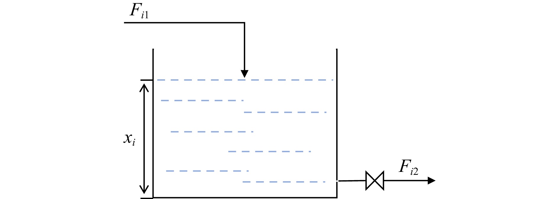
By the mass conservation law, we have s_i\frac{{{d}} x_i}{{{d}} t}=F_{i1}-F_{i2}, for i=1, \ldots, 4 , where s_i is the bottom area of the tank; x_i is the height of the liquid; F_{i1} and F_{i2} are the input and output flows of the tank, respectively. Then, we can obtain
| \dot x_i=\frac{1}{s_i}u_i-f_i | (26) |
where u_i=F_{i1} and f_i=\frac{F_{i2}}{s_i} . Consider the linear valve with disturbance (i.e., F_{i2}=K_ix_i+C_i where K_i is the linear coefficient of the valve and C_i is the constant disturbance). From these, it’s not hard to see that (26) is in line with dynamics (1).
Let s_1=s_2=s_3=s_4=1 , K_1=C_1=0.1 , K_2=C_2=0.2 , K_3=C_3=0.3 , K_4=C_4=0.2 and the initial value be chosen as [x_1(0),x_2(0),x_3(0),x_4(0)]^{{{{{T}}}}}=[5, 0, 2, 1]^{{{{{T}}}}}. Let t_0=0 , \phi(t)= e^{0.2t}-1 . With the designed protocol (2), by simulation, we obtain Fig. 3 which exhibits the trajectories of the closed-loop system signals x_i ’s, u_i ’s, \xi_i ’s and funnel gains \kappa_{i} ’s graph of Fig. 1(b). One can readily see that all the signals are bounded, and particularly, from the first and second subfigures of Fig. 3, the consensus is achieved while the relative states are kept within the prescribed performance boundary.
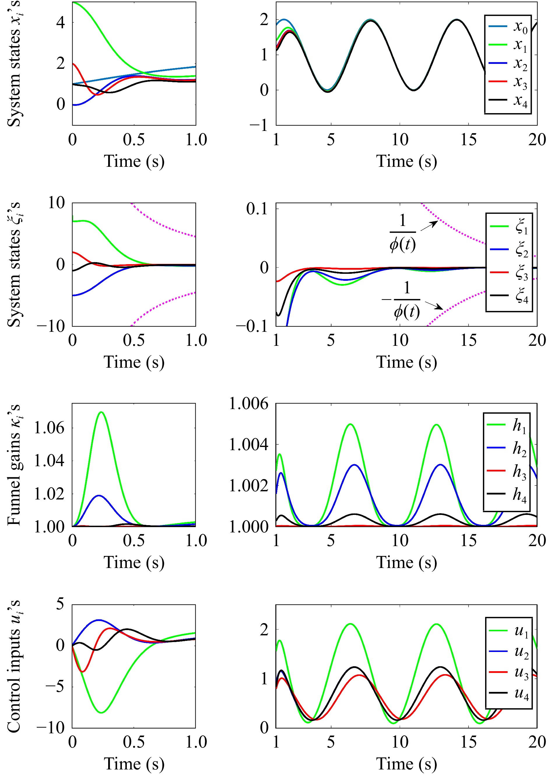
First, aim at the case of MASs where the dynamics of agent is described by (1) with f_1(t,x_1)=x_1(x_1\sin t+1), f_2(t,x_2)= x^2_2\sin t, f_3(t,x_3)=x_3(\sin t+1), f_4(t,x_4)=x_4(x_4\sin t+1) and the control directions are known. Let -g_1=-g_2=g_3=g_4=1 . To illustrate the effectiveness of the designed protocol for any initial values, we conduct the simulation by using “randi([50, 100], 1,4)” to randomly choose [x_1(0),x_2(0),x_3(0),x_4(0)]^{{{{{T}}}}}. Let \phi(t) be the same as the previous example. The following Fig. 4 exhibits the trajectories of the closed-loop system signals graph of Fig. 1(b). Particularly, from the second and third subfigures of Fig. 4, once the relative states approach to the performance boundary, the funnel gains (and hence control inputs) obviously increase, which reflects the control idea of the funnel control.
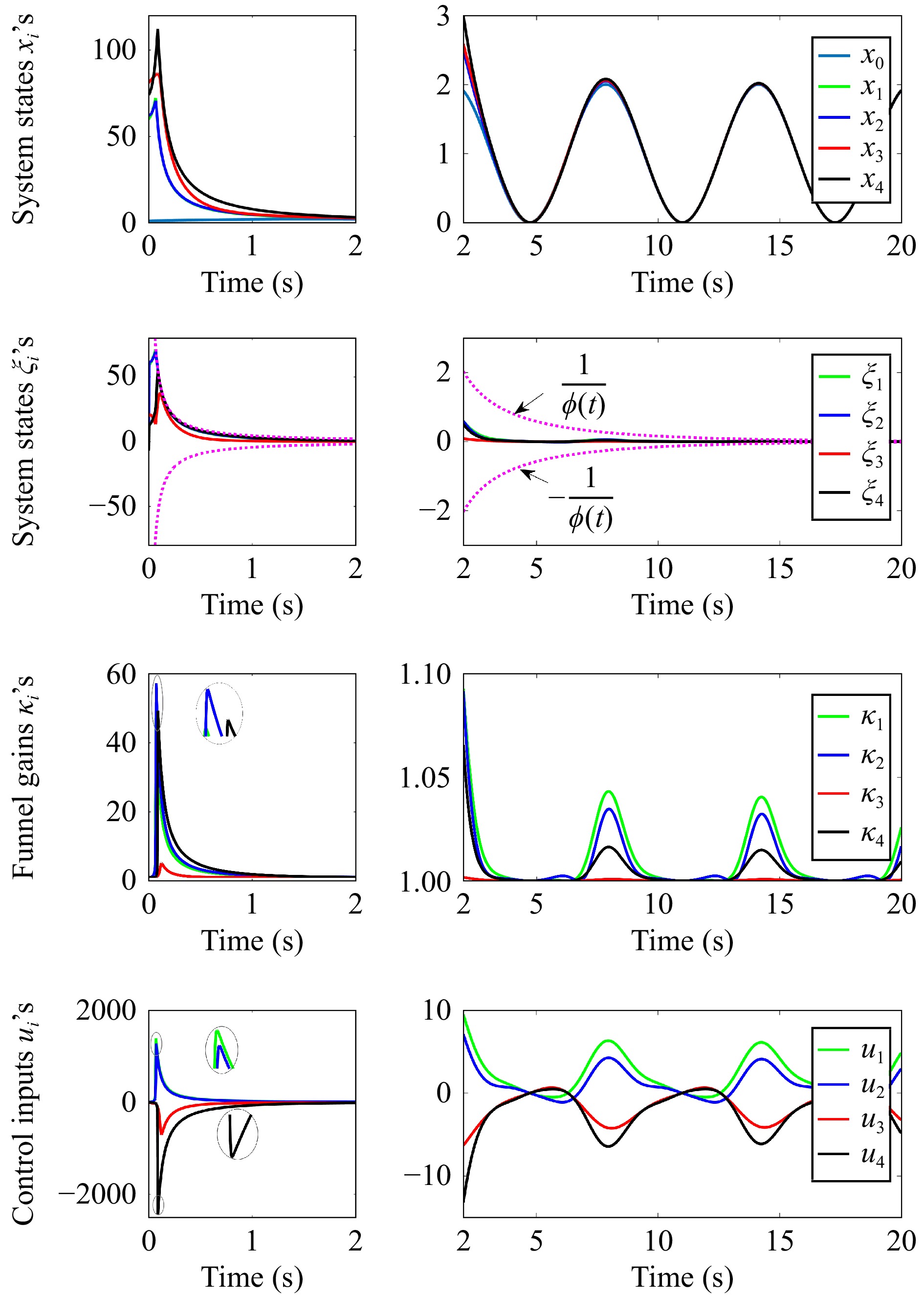
As for the case of MASs with unknown control directions, we choose the same initial values with the practical example. To simulate the unknown control directions, we use “randsrc(1,4)” to randomly generate 1 or −1 for signs of g_i ’s. With protocol (14) and over a hierarchical graph (i.e., of Fig. 1(a)), by simulation, Fig. 5 is obtained and it exhibits the boundedness of closed-loop system signals. Meanwhile, as seen in the first subfigure, consensus is achieved and the second subfigure shows the evolution of relative states within the prescribed performance boundaries.
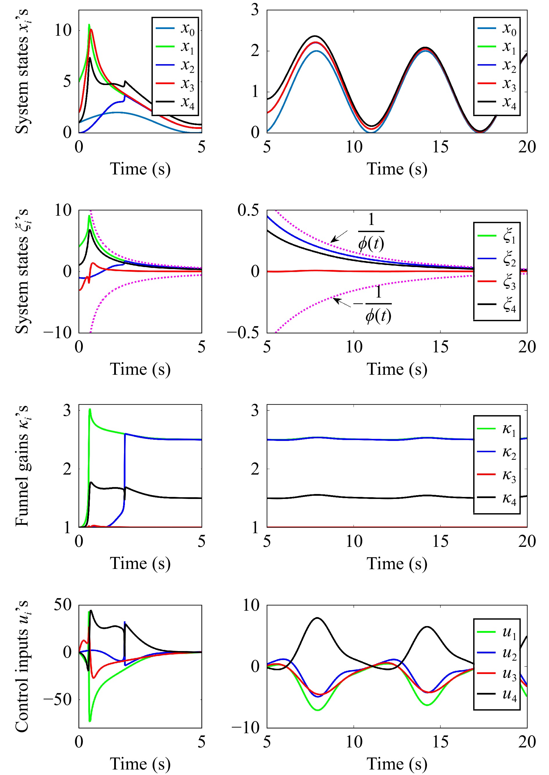
Remarkably, observing the selected system nonlinearities, they cannot be written as the form of \theta_i\phi_i(x_i) as in [21], [24], nor do they (except for f_3(\cdot) ) satisfy the Lipschitz condition as in [23]. This reflects the capability of the proposed approach in dominating more general system nonlinearities. In addition, in the sense of using “randsrc(1,4)” to randomly generate signs of g_i ’s, the control direction of each agent can be nonidentical, which is inherently different from the existing result [19]. Moreover, all control directions rather than partial ones as in [36], are permitted to be unknown.
In the paper, performance-prescribed leader-following consensus has been investigated for MASs typically with heterogeneous unknown nonlinearities and nonidentical unknown control coefficients. Leveraging the powerful FC strategy, fully distributed protocols are designed by incorporating the relative states and funnel gains. Remark that in the designed protocol, an elaborately prescribed time-varying function \phi(t) characterizing the performance boundary, is used to not only construct funnel gains but act as an indispensable part of the protocol, playing a key role in enhancing the control effect to drive consensus errors to zero. When control directions are unknown, a hierarchical graph is considered, essentially simplifying the coupling of control directions. Meanwhile, a smooth function \mathcal{N}(\cdot) equipped with varying signs is introduced to combine with funnel gains for compensating unknowns in the control coefficients. It has been proved that appropriate operations on the graph is helpful for the realizability of consensus facing severe heterogeneities and unknowns.
As for future research, it deserves much effort to develop new strategies for more general MASs that tolerate non-input-matched system nonlinearities or unknown control directions varying with states/time. Moreover, it remains to be studied whether the desired control objectives in the context of unknown control directions can be achieved, without relying on the hierarchical structure of the graph.
| [1] |
A. Jadbabaie, J. Lin, and A. S. Morse, “Coordination of groups of mobile autonomous agents using nearest neighbor rules,” IEEE Trans. Autom. Control, vol. 48, no. 6, pp. 988–1001, Jun. 2003. doi: 10.1109/TAC.2003.812781
|
| [2] |
J. A. Fax and R. M. Murray, “Information flow and cooperative control of vehicle formations,” IEEE Trans. Autom. Control, vol. 49, no. 9, pp. 1465–1476, Sep. 2004. doi: 10.1109/TAC.2004.834433
|
| [3] |
A. Das and F. L. Lewis, “Distributed adaptive control for synchronization of unknown nonlinear networked systems,” Automatica, vol. 46, no. 12, pp. 2014–2021, Dec. 2010. doi: 10.1016/j.automatica.2010.08.008
|
| [4] |
H. Su, G. Chen, X. Wang, and Z. Lin, “Adaptive secondorder consensus of networked mobile agents with nonlinear dynamics,” Automatica, vol. 47, no. 2, pp. 368–375, Feb. 2011. doi: 10.1016/j.automatica.2010.10.050
|
| [5] |
Q. Song, J. Cao, and W. Yu, “Second-order leader-following consensus of nonlinear multi-agent systems via pinning control,” Syst. Control Lett., vol. 59, no. 9, pp. 553–562, Sep. 2010. doi: 10.1016/j.sysconle.2010.06.016
|
| [6] |
H. Zhang and F. L. Lewis, “Adaptive cooperative tracking control of higher-order nonlinear systems with unknown dynamics,” Automatica, vol. 48, no. 7, pp. 1432–1439, Jul. 2012. doi: 10.1016/j.automatica.2012.05.008
|
| [7] |
M. Pirani, E. M. Shahrivar, B. Fidan, and S. Sundaram, “Robustness of leader-follower networked dynamical systems,” IEEE Trans. Control Netw. Syst., vol. 5, no. 4, pp. 1752–1763, Dec. 2018. doi: 10.1109/TCNS.2017.2756346
|
| [8] |
Q. Wei, X. Wang, X. Zhong, and N. Wu, “Consensus control of leader-following multi-agent systems in directed topology with heterogeneous disturbances,” IEEE/CAA J. Autom. Sinica, vol. 8, no. 2, pp. 423–431, Feb. 2021. doi: 10.1109/JAS.2021.1003838
|
| [9] |
F. Chen and D. V. Dimarogonas, “Leader-follower formation control with prescribed performance guarantees,” IEEE Trans. Control Netw. Syst., vol. 8, no. 1, pp. 450–461, Mar. 2021. doi: 10.1109/TCNS.2020.3029155
|
| [10] |
M. Dai, C. K. Ahn, C. Zhang, C. Wei, and J. Wu, “On prescribed performance synchronization to QUAD nonlinear multi-agent network,” IEEE Trans. Circuits Syst. II, Express Briefs, vol. 69, no. 3, pp. 1377–1381, Mar. 2022.
|
| [11] |
W. Wang, D. Wang, Z. Peng, and T. Li, “Prescribed performance consensus of uncertain nonlinear strict-feedback systems with unknown control directions,” IEEE Trans. Syst., Man, Cybern., Syst., vol. 46, no. 9, pp. 1279–1286, Sep. 2016. doi: 10.1109/TSMC.2015.2486751
|
| [12] |
J. Lee, S. Trenn, and H. Shim, “Synchronization with prescribed transient behavior: Heterogeneous multi-agent systems under funnel coupling,” Automatica, vol. 141, p. 110276, Jul. 2022. doi: 10.1016/j.automatica.2022.110276
|
| [13] |
C. Ma and D. B. Dong, “Finite-time prescribed performance timevarying formation control for second-order multi-agent systems with nonstrict feedback based on a neural network observer,” IEEE/CAA J. Autom. Sinica, vol. 11, no. 4, pp. 1039–1050, 2024.
|
| [14] |
I. Katsoukis and G. A. Rovithakis, “Low complexity robust output synchronization protocol with prescribed performance for high-order heterogeneous uncertain MIMO nonlinear multi-agent systems,” IEEE Trans. Autom. Control, vol. 61, no. 6, pp. 3128–3133, Jun. 2022.
|
| [15] |
X. Min, S. Baldi, W. Yu, and J. Cao, “Funnel asymptotic tracking of nonlinear multi-agent systems with unmatched uncertainties,” Syst. Control Lett., vol. 167, p. 105313, Sep. 2022. doi: 10.1016/j.sysconle.2022.105313
|
| [16] |
C. P. Bechlioulis and G. A. Rovithakis, “Decentralized robust synchronization of unknown high order nonlinear multi-agent systems with prescribed transient and steady state performance,” IEEE Trans. Autom. Control, vol. 62, no. 1, pp. 123–134, Jan. 2017. doi: 10.1109/TAC.2016.2535102
|
| [17] |
E. Restrepo and D. V. Dimarogonas, “On asymptotic stability of leaderfollower multi-agent systems under transient constraints,” IEEE Control Syst. Lett., vol. 6, pp. 3164–3169, Jun. 2022. doi: 10.1109/LCSYS.2022.3182846
|
| [18] |
F. Li and Y. Liu, “Control design with prescribed performance for nonlinear systems with unknown control directions and nonparametric uncertainties,” IEEE Trans. Autom. Control, vol. 63, no. 10, pp. 3573–3580, Oct. 2018. doi: 10.1109/TAC.2018.2794886
|
| [19] |
Z. Ding, “Adaptive consensus output regulation of a class of nonlinear systems with unknown high-frequency gain,” Automatica, vol. 51, pp. 348–355, Jan. 2015. doi: 10.1016/j.automatica.2014.10.079
|
| [20] |
Q. Wang and C. Sun, “Distributed asymptotic consensus in directed networks of nonaffine systems with nonvanishing disturbance,” IEEE/CAA J. Autom. Sinica, vol. 8, no. 6, pp. 1133–1140, Jun. 2021. doi: 10.1109/JAS.2021.1004021
|
| [21] |
J. Huang, Y. Song, W. Wang, C. Wen, and G. Li, “Fully distributed adaptive consensus control of a class of high-order nonlinear systems with a directed topology and unknown control directions,” IEEE Trans. Cybern., vol. 48, no. 8, pp. 2349–2356, Aug. 2018. doi: 10.1109/TCYB.2017.2737652
|
| [22] |
W. Wang, C. Wen, J. Huang, and Z. Zheng, “Hierarchical decomposition based consensus tracking for uncertain interconnected systems via distributed adaptive output feedback control,” IEEE Trans. Autom. Control, vol. 61, no. 7, pp. 1938–1945, Jul. 2016. doi: 10.1109/TAC.2015.2479535
|
| [23] |
M. Fan and Y. Wu, “Global leader-following consensus of nonlinear multi-agent systems with unknown control directions and unknown external disturbances,” Appl. Math. Comput., vol. 331, pp. 274–286, Aug. 2018.
|
| [24] |
C. Wang, C. Wen, and L. Guo, “Adaptive consensus control for nonlinear multi-agent systems with unknown control directions and timevarying actuator faults,” IEEE Trans. Autom. Control, vol. 66, no. 9, pp. 4222–4229, Sep. 2021. doi: 10.1109/TAC.2020.3034209
|
| [25] |
J. Peng, K. Wang, C. Li, and S. Xiao, “Prescribed performance control of multiple parametric strict-feedback systems in the presence of unknown control directions,” IEEE Trans. Syst., Man, Cybern., Syst., vol. 54, no. 1, pp. 265–274, Jan. 2024. doi: 10.1109/TSMC.2023.3308217
|
| [26] |
A. Ilchmann, E. P. Ryan, and C. J. Sangwin, “Tracking with prescribed transient behaviour,” ESAIM Control Optim. Calc. Var., vol. 7, pp. 471–493, Sep. 2002. doi: 10.1051/cocv:2002064
|
| [27] |
M. Nagy, Z. Akos, D. Biro, and T. Vicsek, “Hierarchical group dynamics x in pigeon flocks,” Nature, vol. 464, pp. 890–893, Apr. 2010. doi: 10.1038/nature08891
|
| [28] |
J. Peng and X. Ye, “Cooperative control of multiple heterogeneous agents with unknown high-frequency-gain signs,” Syst. Control Lett., vol. 68, pp. 51–56, Jun. 2014. doi: 10.1016/j.sysconle.2014.02.010
|
| [29] |
J. Sang, D. Ma, and Y. Zhou, “Group-consensus of hierarchical containment control for linear multi-agent systems,” IEEE/CAA J. Autom. Sinica, vol. 10, no. 6, pp. 1462–1474, Jun. 2023. doi: 10.1109/JAS.2023.123528
|
| [30] |
K. Li, K. Zhao, and Y. Song, “Adaptive consensus of uncertain multiagent systems with unified prescribed performance,” IEEE/CAA J. Autom. Sinica, vol. 11, no. 5, pp. 1310–1312, May 2024. doi: 10.1109/JAS.2023.123723
|
| [31] |
P. N. Shivakumar and K. H. Chew, “A sufficient condition for nonvanishing of determinants,” Proc. Amer. Math. Soc., vol. 43, no. 1, pp. 63–66, Mar. 1974. doi: 10.1090/S0002-9939-1974-0332820-0
|
| [32] |
Z. Qu, Cooperative Control of Dynamical Systems: Applications to Autonomous Vehicles, London, UK: Springer-Verlag, 2009.
|
| [33] |
J. K. Hale, Ordinary Differential Equations, 2nd ed., New York, USA: Wiley-Interscience, 1980.
|
| [34] |
H. Shao, L. Pan, M. Mesbahi, Y. Xi, and D. Li, “Distributed neighbor selection in multi-agent networks,” IEEE Trans. Autom. Control, vol. 68, no. 11, pp. 6711–6726, Nov. 2023. doi: 10.1109/TAC.2023.3246425
|
| [35] |
J. Shen, “Cucker-smale flocking under hierarchical leadership,” SIAM J. Appl. Math., vol. 68, no. 3, pp. 694–719, Mar. 2008. doi: 10.1137/060673254
|
| [36] |
J. Chen, J. Li, W. Chen, S. Zhang, and J. Zhang, “Iterative learning control for nonlinear uncertain parameterized multi-agent systems with non-identical partially unknown control directions,” IEEE Trans. Netw. Sci. Eng., vol. 11, no. 4, pp. 3358–3369, Jul.–Aug. 2024.
|

Figures(5)


L. Yu and Y. Liu, “Compensation for heterogeneous unknowns and performance-prescribed consensus,” IEEE/CAA J. Autom. Sinica, vol. 12, no. 1, pp. 173–182, Jan. 2025. doi: 10.1109/JAS.2024.124794
 DownLoad:

 DownLoad:


