A journal of IEEE and CAA , publishes high-quality papers in English on original theoretical/experimental research and development in all areas of automation
A. Benyahia, M. Stanković, R. Madonski, O. Babayomi, and S. Manojlović, “Improving control performance by cascading observers: Case of ADRC with cascade ESO,” IEEE/CAA J. Autom. Sinica, 2024. doi: 10.1109/JAS.2024.124995
Citation: A. Benyahia, M. Stanković, R. Madonski, O. Babayomi, and S. Manojlović, “Improving control performance by cascading observers: Case of ADRC with cascade ESO,” IEEE/CAA J. Autom. Sinica, 2024. doi: 10.1109/JAS.2024.124995

Improving Control Performance by Cascading Observers: Case of ADRC With Cascade ESO

doi: 10.1109/JAS.2024.124995
Funds:  The work was partially supported by the project of the University of Defence in Belgrade, Serbia (VA/TT/1/25-27)
More Information
  • In this paper, we show the performance benefits of connecting multiple observers within a control system. We focus here on a particular observer-based control approach, namely the active disturbance rejection control (ADRC) with cascade extended state observer (ESO). For this framework, we analyze the control performance in terms of quality of observer estimation, reference tracking, disturbance rejection, sensitivity to measurement noise/unmodeled dynamics, and overall stability. A comprehensive frequency response analysis is performed to study the influence of cascading the observers on the selected quality criteria. To make the inquiry beneficial also to practitioners, FPGA-in-the-loop tests are conducted using a guided missiles gimbaled seeker. They validate the theoretical findings in discrete-time settings, where the sampling time and hardware resource requirements become a factor. The results of the investigation are distilled into guidelines for prospective users on when and how a cascade observer structure can be useful for controls.


  • DRIVEN by industrial challenges requiring control frameworks that go beyond conventional PID controllers, techniques based on the methodology of active disturbance rejection control (ADRC) were proposed as a potential alternative [1]. Their primary objective is to counteract the effect of disturbances on the system dynamics by actively estimating and compensating them in a unified manner. Such an online disturbance rejection capability is a hallmark of ADRC, making it a pragmatic choice across a spectrum of applications [2]. At its core, the effectiveness of ADRC against disturbances is intricately linked to the performance of its key component—extended state observer (ESO). It provides the estimates of disturbances and system states for controller implementation. In fact, ESO’s most desirable characteristic is the ability to estimate low-to-medium-frequency disturbances (up to its bandwidth) while also attenuating measurement noise [1]. However, due to its intrinsic high-gain structure, disturbance rejection is often achieved at the expense of its noise attenuation performance.

    It may appear intuitive to mitigate the noise effect simply by integrating a low-pass filter (LPF) in the control structure. However, as shown in [3], the LPF may inadvertently compromise the system robustness if not carefully placed and tuned. Therefore, the use of LPF should be approached with caution and with the well-established and well-understood stability of the entire closed-loop system, including the LPF.

    To address the issue of limited ADRC performance due to the presence of non-negligible sensor noise, the concept of cascading the observers started to be exploited in the literature. The goal was to use several working observers to attenuate high-frequency noise while simultaneously preserving tracking quality and disturbance rejection capabilities. To this effect, different cascade approaches were proposed. In [4], for example, a cascade structure of high-gain conventional ESOs was introduced that connected the observers in series and with saturation function between them to reduce the gain order. In contrast, the so-called cascade ESO structure (CESO), introduced by Łakomy and Madonski in [5], suggested a different configuration to filter out high-frequency measurement noise. The idea was that each ESO in the cascade operates within a specific frequency range enabling the reconstruction of the total disturbance in a piece-wise manner, under the condition that the first ESO operates within the lowest possible frequency to prevent amplifying noise. This configuration not only enhanced the robustness of the system but also improved the tracking accuracy. The efficacy of cascade configuration of observers within the ADRC framework was eventually found to be not only an interesting theoretical exercise but also lead to tangible practical solutions with experimental implementations in various fields, including power electronics [6], [7], and automotive applications [8].

    Building on the results from CESO, [9] provided a guideline for selecting the number of cascade levels based on the expected nature of the disturbance, which helps with the practical implementation of CESO. The study also highlights the limitation of CESO in numerical implementation due to its high-order gains and proposes a low-power high-gain ESO as a solution. However, the disturbance rejection capabilities are not further improved. In response to that, the concept of CESO was extended to a multi-frequency ESO framework that incorporates different ESO architectures including a cascade of hybrid [10] and parallel [11] sub-ESOs. It considers the total disturbance as a periodic function modeled with a Fourier series, where each component is approximated using the Taylor series. Consequently, in [10], the proposition of a hybrid cascade structure with combined parallel sub-ESOs proved better disturbance rejection than CESO. Although it inherits the beneficial noise suppression features of the CESO under specific conditions, its higher level showed relatively lower noise rejection than the CESO. Additionally, the study lacked a generalized guideline for selecting the number of sub-frequencies and added more extra design parameters to be tuned. Authors of [12] proposed a hybrid parallel-cascade structure, thus overcoming limitations of conventional adaptive gain in [10] and [11]. Most recently, the unified interpretation of CESO and the generalized ESO was investigated in [13].

    As the above overview of selected works indicates, the predominant focus so far has been on enhancing noise and disturbance rejection capabilities, overshadowing other fundamental closed-loop performance factors such as stability margins, sensitivity to unmodeled dynamics, and discrete-time implementation, where sampling time and hardware resource requirements are key factors. Despite various advancements, this fundamental trade-off between noise suppression and disturbance rejection persists. However, from our perspective, the question does not lie in further improving noise and disturbance rejection concurrently; rather, in identifying the optimal structure that can deliver peak performance across various dimensions, aligning with the primary control objective. The contributions of this paper are thus as follows.

    1) A comprehensive frequency domain analysis of ADRC with CESO. The analysis evaluates key performance parameters such as observer estimation quality, reference tracking, disturbance rejection, sensitivity to measurement noise/unmodeled dynamics, and overall stability. The results are distilled into guidelines for future users interested in understanding the benefits and limitations of cascading the observers.

    2) Bridging the gap between theoretical insights and practical implementation through FPGA-in-the-loop (FIL) validation tests. They are carried out on a three-axis gimbaled seeker platform, offering a real-world perspective and considering crucial factors like sampling time and hardware resource requirements.

    This paper is not focused on proving the superiority of one cascade structure over the other nor on introducing a new one. Our motivation is to comprehensively study the impact of adding a cascade structure to a control system. That includes understanding the advantages and limitations of such a procedure. Since we are investigating the above question from a particular perspective of ADRC, the next section provides a brief review of the ADRC framework as well as the theory of ESO and its cascade version in order to have a single, convenient point of reference for later deliberations.

    In the paper, we consider a class of second-order single input single output (SISO) dynamical systems, frequently encountered in engineering applications, described by

    ¨y=a0y+a1˙y+bu+d
    (1)

    where y=y+η is the measured output corrupted with sensor noise η, y is the system’s output, u is the control input, a0 and a1 are the system uncertain internal parameters, d refers to the external disturbance affecting the system behavior, and b=b0+Δb, with b0 being a rough approximation of b and Δb its associated uncertainty.

    The control objective is to force the output of the system y to follow a reference signal r despite the presence of external disturbance d, model uncertainties related to a0,a1 and Δb as well as high-frequency noise n corrupting the system output. We also make the following practical assumptions:

    A1) The reference signal r and its derivatives are bounded.

    A2) Neither r nor its derivatives are known in advance.

    A3) The external disturbance d is bounded.

    A4) The output signal y is the only measurable signal.

    To achieve the above control objective, (1) could be expressed in the framework of ADRC in a compact form:

    ¨y=f+b0u
    (2)

    where f=a0y+a1˙y+Δbu+d denotes the so-called total disturbance, aggregating both the internal and external disturbances. The absence of any prior information on the reference signal r except its boundness (assumptions A1 and A2) leads to reformulation of (2) in error domain:

    ¨e=fb0u
    (3)

    where ery is the tracking error and f=¨rf is now the total disturbance in error domain.

    Remark 1: A comparison of key characteristics of output- and error-based ADRC is comprehensively described in [14].

    The desired closed-loop performance could be achieved by applying the following control law:

    u=(u0+ˆf)/b0=(k0ˆe+k1ˆ˙e+ˆf)/b0
    (4)

    where [k0 k1]T=[ω2c 2ωc]T are the controller gains calculated by placing the poles of the closed-loop error dynamics at ωc (controller bandwidth), which is a popular simplifying tuning approach especially useful in practice, e.g., [15]. Term u0=k0ˆe+k1ˆ˙e is a simple proportional-integral feedback stabilizing control. Looking at (4), the required estimates ˆe,ˆ˙e,ˆf need to be estimated, for example with a dedicated observer.

    By considering f as an additional state variable, a state vector x=[x1 x2 x3]T=[e ˙e f]T can be used to represent system (3) in its extended state form:

    {˙x=Ax+Bu+H˙fe=CTx
    (5)

    where A=[02×1I2×2001×2], B=[0 b0 0]T, C=[1 0 0]T, and H=[0 0 1]T. The following ESO can be then designed:

    {˙ˆx=Aˆx+Bu+L[eCTˆx]ˆe=CTˆx
    (6)

    where ˆx=[ˆx1 ˆx2 ˆx3]T=[ˆe ˆ˙e ˆf]T and L=[l1 l2 l3]T with lj=(3j)ωjo are the observer gains tuned by placing poles of the closed-loop dynamics at ωo (observer bandwidth).

    The CESO was initially introduced and theoretically proved in [5] and, as shown in Fig. 1, is a series of p number of interconnected observers, which usually takes the form:

    Figure  1.  The ADRC scheme with p-level CESO (variation of a block diagram from [5]).
    {˙ξ1=Aξ1+Bu+L1[eCTξ1]˙ξi=Aξi+B(uHTb0i1j=1ξj)+LiCT[ξi1ξi],  fori{2,,p}
    (7)

    where ξi=[ξ(1,i) ξ(2,i) ξ(3,i)]T, for i{1,,p}, is the state vector of each cascade level and Li=[l(1,i) l(2,i) l(3,i)]T where l(j,i)=(3j)ωjoi are the associated observer gains. The bandwidth of each level is also parameterized by ωo, here as ωoi=αipωo with α>1. Finally, the estimates used to calculate the control signal (4) are then obtained as

    ˆz=[ˆz1 ˆz2 ˆz3]T=ξp+HHTp1j=1ξj.
    (8)

    The underlying concept of CESO is that the first observer in the cascade estimates the extended state vector primarily relying on the noise-corrupted output y. The first observer is tuned with the lowest bandwidth ωo1 to deliver sufficiently accurate estimates and at the same time prevent amplifying high-frequency measurement noise. Subsequently, each of the succeeding observers i within the cascade, namely (i2), characterized by a higher bandwidth ωoi>ωo(i1), estimates further the total disturbance residue ˆfi relying on the noise-filtered output ξi1 of the previous observer. The estimated total disturbance is then the sum of the estimated residues in each level given by ˆf=pi=1ˆfi=HTpi=1ξi.

    Remark 2: For p=1, we get ESO as seen in Section II-C.

    The frequency analysis is carried out by deriving various transfer functions for the 1-level (single ESO, no cascade) and p-level CESOs with p{2,...,5}.

    Remark 3: In practice, for the second-order systems, the level of CESO is limited to 2p4 due to increased complexity that does not justify the obtained performance increase, as shown in [16]. Therefore, without loss of generality, this study is constrained to CESO structures up to the level p=5.

    Following that, and to ensure an objective comparative analysis between the five CESO structures, the tuning methodology adopted in this work adheres to the following guidelines:

    1) ωo1 needs to be sufficiently large to ensure robustness, yet small enough to filter out measurement noise;

    2) ωo(i1) should be set small enough to preserve the total disturbance estimation residue, which can then be estimated by the subsequent cascade level with a bandwidth ωoi> ωo(i1). For instance, ωoi is chosen as illustrated in Table I (approach from [5]), reducing the tuning parameters to just two (ωo and α) regardless of the number of levels p;

    Table  I.  Bandwidth Parameterization of CESO (Approach From [5] Extended Here to a General p-Order Case)
    CESO level ωo1 ωo2 ωo3 ωop
    1 ωo
    2 ωoα ωo
    3 ωoα2 ωoα ωo
    p ωoαp1 ωoαp2 ωoαp3 ωo
     | Show Table
    DownLoad: CSV

    3) ωc is constant for each of the ADRC structures.

    The state estimation quality of the CESO structures is evaluated based on the frequency response analysis. Assuming u=0, the transfer function between the estimation error ˜ej(s)Zj(s)^Zj(s) of the j-th estimated state ^Zj(s) and the total disturbance F(s) in frequency domain is obtained by applying a Laplace transform to (7), and its form for the 1-level CESO (ESO) is given as follows:

    G1ej(s)={s(s+ωo)n+1j1k=1l(k)sj(k+1),if  2jn+1s(s+ωo)n+1,if  j=1
    (9)

    and for a p-level CESO (p2) as

    G(p)ej(s)=sjΦp(s)+spΨ(j,p)(s)pk=1(s+ωok)n+1,1jn+1
    (10)

    where n=2 is the system’s order, i,pZ+, and Φp(s)= k=0cksk,Ψ(i,p)(s)=k=0qksk are polynomials satisfying c00,q00.

    Theorem 1: For a second-order system (n=2) subjected to polynomial-like disturbances in the form F(s)=mk=1fksk, where mZ+, a p-level CESO achieves asymptotic convergence in estimating the j-th state if and only if mminjn+1(j,p). Therefore, for optimal disturbance rejection, the observer level p should satisfy p=n+1.

    Proof: Consider the CESO defined by (7), and let ζ(s),Z(s),E(s),U(s),F(s) be the Laplace transform of ξ,z,e,u and f respectively. The estimation error for the j-th component Zj(s), denoted by ˜ej(s) for 1jn+1, is given by

    ˜ej(s)=Zj(s)ˆZj(s)=sj1E(s)ˆZj(s).
    (11)

    Case 1 (p=1): First, let us examine the 1-level CESO (ESO) case. From (8), when p=1, we have ˆZj(s)=ζ(j,1)(s). Applying Laplace transform to (7), ˆZj(s) takes form:

    ^Zj(s)={sjsn+2[n+1k=jl(k,1)sn+1k˜e1(s)b0sU(s)],if  1jnl(n+1,1)s˜e1(s),if  j=n+1.
    (12)

    Assuming U(s)=0 and applying the Laplace transform to (3), leads to F(s)=snE(s) and from (12) ^Zj(s) can be expressed in the following compact form:

    ^Zj(s)=sjsn+2n+1k=jl(k,1)sn+1k˜e1(s),1jn+1.
    (13)

    By substituting (13) into the estimation error (11), the transfer function for the j-th estimated component G1ej(s)= ˜ej(s)/F(s), is calculated as follows:

    G1ej(s)=sjsn+2[sn+1k=jl(k,1)sn+1kG1e1(s)],1jn+1.
    (14)

    Note that (s+ωo1)n+1=n+1k=0l(k,1)sn+1k and ωo1=ωo. After simplification, G1e1(s)=s(s+ωo1)n+1 and therefore, G1ej(s) can be expressed as

    G1ej(s)=s(s+ωo)n+1j1k=0l(j,1)sj(k+1),1jn+1.
    (15)

    Case 2 (p>1): A p-level CESO consists of a cascade of p ESOs. Let ˜e(1,i)(s) be the estimation error for the first component of the i-th ESO in the cascade expressed as

    ˜e(1,i)(s)={ˆζ(1,i1)(s)ˆζ(1,i)(s),if  1ipE(s)ˆζ(1,1)(s)if  i=1.
    (16)

    From (8), the j-th estimated component ˆZj(s) is expressed in terms of ˆζ(j,p)(s) as

    ˆZj(s)={ˆζ(j,p)(s),if  1jnpi=1ˆζ(n+1,i)(s),if  j=n+1
    (17)

    where ˆζ(n+1,i)(s)=l(n+1,i)s˜e(1,i)(s).

    Using the same logic in (12) by applying the Laplace transform to (7), the j-th estimated state ˆζ(j,p)(s) of the p-th ESO can be expressed as follows:

    ˆζ(j,p)(s)={sjsn+2[n+1k=jl(k,p)sn+1k˜e(1,p)(s)b0sUp(s)],if  1jnl(n+1,p)s˜e(1,p)(s),if  j=n+1
    (18)

    where Up(s)=U(s)1b0p1j=1ˆζ(n+1,j)(s).

    Assuming U(s)=0 and substituting (18) back in (17), ˆZj(s) can be expressed in the form:

    ˆZj(s)=sjsn+2[A(j,p)(s)˜e(1,p)(s)+p1k=1l(n+1,k)˜e(1,k)(s)],1jn+1
    (19)

    where A(j,p)(s)=n+1k=jl(j,p)sn+1k.

    Therefore, substituting (19) in (11) yields the transfer function G(p)ej(s) relating the estimation error ˜ej(s) of the p-level CESO to the total disturbance F(s), with F(s)=snE(s):

    G(p)ej(s)=sjsn+2[sA(j,p)Ge(1,p)(s)p1k=1l(n+1,k)Ge(1,k)(s)],p2.
    (20)

    The term Ge(1,p)(s)=˜e(1,p)(s)/F(s) denotes the transfer function relating ˜e(1,p)(s) to F(s) for the first component of the p-th ESO in the cascade. Using (16) and (18), under the assumption U(s)=0, Ge(1,p)(s) results in

    Ge(1,p)(s)={s(s+ωo1)n+1pk=2[A(1,k1)(s+ωok)n+1],if  p2s(s+ωo1)n+1,if  p=1
    (21)

    where A(j,i)(s)=nk=jl(j,i)sn+1k.

    Remark 4: For p=1, we obtain ESO, leading to Ge(1,1)(s)=G1e1(s), which has already been calculated in (14).

    By substituting (21) into (20), we have

    G(p)ej(s)=sjΦp(s)+spΨ(j,p)(s)pk=1(s+ωok)n+1,1jn+1
    (22)

    where Φp(s),Ψ(j,p)(s) are polynomials expressed in the following form:

    Ψ(j,p)(s)={0,if , j=1(j1k=1l(k,p)sj1k)p1m=2(nk=1l(k,m1)snk),if  2jnpm=1(nk=jl(k,m)snk),if  j=n+1
    Φp(s)=p1k=2(k1m=1A(1,m)(s)pm=k+1(s+ωom)n+1)+pm=2(s+ωom)n+1+p1m=1A(1,m)(s).

    Applying the second limit theorem of the Laplace transform to (22) and (15), the steady-state total disturbance estimation error is, for 1jn+1:

    limtej(t)=lims0sG(p)ej(s)F(s).
    (23)

    For polynomial-like disturbances in the form of F(s)= mk=1fksk, mZ+, the condition for achieving asymptotic convergence can be expressed as

    limtej(t)=0m=minjn+1(j,p)
    (24)

    where p,nZ+.

    In terms of the total disturbance reconstruction performance, observers with (p3) are equivalent to higher-order ESOs with one, two, and three extended state variables, respectively [17]. However, raising the CESO level beyond p=3 does not improve the quality of disturbance estimation for higher-order disturbances (m3).

    Choosing the observers’ bandwidths as shown in Table I, the frequency responses magnitude plots of the obtained transfer functions (9) and (10), are presented in Figs. 2(a) and 2(b). From Fig. 2(a), all CESO structures (p2) outperform the conventional ESO (p=1), showcasing enhanced total disturbance estimation capabilities. Notably, a nonlinear relationship is observed between the CESO level p and the disturbance rejection estimation error e3, leading to an optimal total disturbance estimation within the third CESO structure (p=3). This nonlinear behavior is attributed to the tuning of the interconnected ESOs in the cascade (ωoi=αipωo).

    Figure  2.  Estimation quality in frequency domain.

    Further, from Fig. 2(b), and due to the lower gains of the first observer in the cascade relative to conventional ESO (see Table I), the estimation quality of ˙e and especially e is degraded for a higher level (p2). However, it should be noted that it does not affect closed-loop control performances if the control law (4) is synthesized by the measured error e instead of its estimation ˆe.

    The closed-loop tracking performance, disturbance rejection, noise sensitivity and robustness of the proposed CESO-based ADRC algorithm with different levels of p are compared by numerical simulation in the frequency domain. The considered control system is presented in the transfer function form as shown in Fig. 3, where the terms R(s),E(s),D(s),U(s),N(s), and Y(s) are Laplace transforms of reference signal, control tracking error, external disturbance, control signal, noise, and output, respectively.

    Figure  3.  Transfer function representation of ADRC with CESO.

    The analyses are carried out on the generic second order plant model P(s) which can be considered as linearized model of the introduced general nonlinear dynamic system (1): P(s)=1s2+s+1. The transfer functions of the CESO-based ADRC controllers Gc(p)(s)=U(s)/E(s) for p={1,,5} are obtained from (7) applying Laplace transforms with the use of the real error e instead of ˆe in the control law (4).

    Gc(p)(s)=3pi=0apisib0s3p1j=0bpjsj.
    (25)

    The controllers are tuned based on the pole-placement method, such that the observer bandwidths are set according to Table I, and the closed-loop system bandwidth ωc=2 rad/s is used for all the control structures. By choosing b0=1, the full knowledge of the plant gain is assumed.

    1) Tracking and disturbance rejection: To evaluate tracking and external disturbance rejection performances, the transfer functions from reference R(s) to tracking error E(s), and from external disturbance D(s) to the output Y(s), are derived respectively as follows, assuming M(s)=Gc(p)(s)P(s):

    GER(s)=1M(s)1+M(s),GYD(s)=P(s)1+M(s)
    (26)

    with their magnitude responses shown in Fig. 4(a). The obtained results indicate the superior performance of CESO-based structures (p2) compared to the standard ESO-based control system within the low-frequency range (lower than ωc). Significantly, the optimal performance is attributed to the third CESO structure, as it provides the overall most accurate estimation of the system’s states. At the high-frequency range, the minimal difference implies similar tracking and disturbance rejection performance. Another possible reason for poor tracking and disturbance rejection at p>3 is that the selected bandwidth parameters for the higher cascade levels may not be optimal for good tracking and disturbance estimation. Further study (beyond the scope of this work) is needed on optimal CESO parameter tuning/design to achieve improved performance for p>3 cascade levels.

    Figure  4.  Closed-loop control performance in frequency domain.

    2) Noise sensitivity: The measurement noise sensitivity is analyzed based on the frequency response of the transfer function from the measurement noise N(s) to the control signal U(s), which is defined as

    GUN(s)=Gc(p)1+M(s).
    (27)

    The magnitude frequency response plots of the (27) for the considered control systems are presented in Fig. 4(b).

    It can be noted that the behaviour of the GUN(s) at high frequencies is of primary importance in the noise sensitivity analysis, since the measurement noise is mainly concentrated in this frequency range. Therefore, from Fig. 4(b), one can note that with increasing cascade level p the control systems achieve significantly better noise attenuation properties.

    3) Stability margins: To analyze the stability and robustness of the proposed control systems, positive and negative gain margins (GM+, GM) and phase margin (PM) were calculated and tabulated in Table II.

    Table  II.  Gain and Phase Margins of the Closed-Loop System
    CESO GM+ GM PM
    p=1 18.92   70.01
    p=2 10.42 −32.95 41.61
    p=3 8.01 −12.79 33.56
    p=4 8.80 −18.35 39.82
    p=5 12.2 −19.54 54.03
     | Show Table
    DownLoad: CSV

    Consequently, as observed in Table II, the minimum stability margins of the considered closed-loop system are associated with CESO of level p=3. This particular configuration also aligns with the optimal tracking accuracy and disturbance rejection performance among all other CESO structures. This observation underscores the inherent trade-off between stability margins and system performance, wherein the system achieves the best tracking accuracy and disturbance rejection at the expense of reduced stability margins.

    4) Unmodeled dynamics sensitivity: To analyze the robustness of the considered control structure in the presence of unmodeled dynamics, the closed-loop system stability margins are obtained by adding a second-order dynamics ω2n/(s2+2ξωns+ω2n) in cascade with the plant model P(s). The damping factor is adopted as ξ=0.707 and the natural frequency of unmodeled dynamics is taken as: ωn={α2ωo,α1ωo,ωo,αωo,α2ωo}.

    The obtained stability margins are gathered in Table III. In alignment with the findings presented in Section III-B-3), it is clear that as the natural frequency ωn decreases relative to ωo, the impact of unmodeled dynamics on the closed-loop stability intensifies. The higher order CESOs (p>3) proved more robust to the presence of unmodeled frequency dynamics. This robustness is attributed to the incorporation of more additional ESOs operating at lower frequencies than ωn. On the other hand, with the increase of ωn (ωn>ωo), the impact of unmodeled dynamics decreases, and the stability margins for all considered observer structures increase and approach the values without unmodeled dynamics (shown in the Table II).

    Table  III.  Gain and Phase Margins in the Presence of Unmodeled Dynamics, Where “*” Denotes Unstable Behavior
    Metric CESO Unmodeled dynamics frequency ωn
    ωo9 ωo3 ωo 3ωo 9ωo
    GM+ p=1 * * 6.33 11.86 15.71
    p=2 * * 2.73 7.22 9.21
    p=3 * * 3.54 6.39 7.45
    p=4 * 2.41 6.38 7.94 8.51
    p=5 4.26 8.67 10.85 11.72 12.03
    GM p=1 * *      
    p=2 * * −30.96 −32.34 −32.75
    p=3 * * −11.27 −12.32 −12.64
    p=4 * −16.57 −17.79 −18.17 −18.29
    p=5 −18.12 −19.08 −19.39 −19.49 −19.52
    PM p=1 * * 42.41 60.99 67.01
    p=2 * * 13.91 32.58 38.61
    p=3 * * 15.98 27.77 31.63
    p=4 * 12.68 30.96 36.88 38.84
    p=5 25.16 44.63 50.91 52.99 53.68
     | Show Table
    DownLoad: CSV

    In practical implementation, the performance of discrete-time CESO structures is linked to the proper choice of sampling time Ts. The influence of Ts on the controller’s stability margins serves as a critical parameter that must be investigated to ensure proper functioning in real-world applications. Given this, the discrete-time transfer functions of the controller with different CESO’s structures p{1,,5} were obtained through a practical numerical approach. Specifically, by discretizing the continuous-time transfer functions (25) using zero-order hold method for a range of values of Ts. This empirical approach effectively captured the discrete-time behavior of the controller without relying on symbolic discretization.

    As anticipated, from Table IV, in the case of a high sampling rate, the CESO-based control system behaves similarly to its continuous counterpart. However, as we transition to lower sampling rates, the effect of discretization can be evident with a marked degradation in gain margins, shown in Fig. 5(a), as well as in phase margins, shown in Fig. 5(b).

    Table  IV.  Gain and Phase Margins for Continuous- and Discrete-Time CESO, Where “*” Denotes Unstable Behavior
    Metric CESO Contin. Discrete (with various Ts)
    106 104 5103 102 2.5102
    GM+ p=1 18.90 18.90 17.75 13.68 * *
    p=2 10.41 10.41 10.02 * * *
    p=3 8.01 8.01 7.83 0.81 * *
    p=4 8.81 8.81 8.71 5.09 1.65 *
    p=5 12.20 12.20 12.15 10.08 8.51 4.16
    GM p=1         * *
    p=2 −32.95 −32.95 −32.89 * * *
    p=3 −12.03 −12.79 −12.74 −10 * *
    p=4 −18.35 −18.35 −18.33 −17.43 −16.9 *
    p=5 −19.54 −19.54 −19.54 −19.28 −19.09 −18.03
    PM p=1 70.69 70 69.08 40.87 * *
    p=2 41.60 40.68 40.68 * * *
    p=3 33.56 33.56 32.97 3.43 * *
    p=4 39.82 39.52 39.52 24.95 8.92 *
    p=5 54.03 53.92 53.92 48.69 43.55 24.11
     | Show Table
    DownLoad: CSV
    Figure  5.  Relation between minimum stability margins in discrete- (GMD, PMD) and continuous-time (GMC, PMC).

    By analyzing the drop rate in stability margins, it is observed that the rate of decrease in gain margin slows down with increasing p. Although the phase margin of the conventional ESO (p=1) is comparatively less affected by variations in sampling time when compared to the 2-level and 3-level CESOs, a similar trend is observed for higher-level CESOs with p2, extending the pattern observed in gain margin.

    This suggests a more robust performance of higher-level CESO under lower sampling conditions. Due to this, the additional complexity of a higher-level CESO could be justified, given its potential to better preserve the system’s stability in the face of low sampling rates.

    The results of the performed frequency-domain analysis can be summarized as follows.

    1) Disturbance rejection and tracking accuracy improve with higher cascade levels up to p=3. Above p=3, further study is necessary to determine how to optimally design sub-bandwidths at the cascaded levels for improved disturbance rejection and estimation accuracy.

    2) Noise attenuation generally increases with the number of cascade levels.

    3) Stability margins decrease as disturbance estimation and tracking accuracy improve.

    4) Robustness to low-frequency unmodeled dynamics improves as the cascade levels increase. In contrast, for high-frequency unmodeled dynamics, robustness decreases as the cascade levels increase up to p=3, followed by an improvement for p=4 and p=5.

    5) More robust performance is obtained at lower discretization sampling times as the cascade levels increase.

    In the following part, the validity of these observations from the theoretical analysis will be checked in a more practical environment utilizing a hardware in a loop setup.

    The gimbaled seeker represents a vital component in a missile guidance system responsible for locating and tracking the target by providing data for guiding the missile toward the target. The seeker’s performance relies heavily on the precise control of its three-axis platform. Throughout the missile’s cruise, this platform is subjected to disturbances resulting from high velocity and torques induced by air stream (known as disturbance torque), as well as noise from the seeker’s optoelectronic/radar system, external electromagnetic interference or countermeasures generated by the target (jamming).

    Therefore, the objective of this section is to verify whether the performance of the considered CESO-based ADRC structures p={1,2,3} holds under these high noise and disturbance conditions. The choice of these specific CESO structures is based on the results gathered in the theoretical part. Here, FPGA-in-the-loop (FIL) validation tests on a three-axis gimbaled seeker platform are performed. The FIL test methodology presented in Fig. 6 for control algorithm implementation, prototyping, and validation is based on low-cost FPGA chip and MATLAB/Simulink software.

    Figure  6.  The used FPGA-in-the-loop (FIL) test setup.

    The hardware description language (HDL) code of the proposed CESO-based control structures is generated using MATLAB/Simulink HDL Code Generation toolbox, based on the controller’s discrete form realized in a fixed-point representation format. Then, following the MATLAB/Simulink FIL wizard, the controller FIL block is formed by choosing the desired FPGA target platform; in this case, a low-cost Basys 3 board with Xilinx Artix 7 FPGA chip XC7A35T is used. The generated controller FIL block is included in the control loop of the three-axis model realized in MATLAB/Simulink. By running the simulation, the controller is implemented in the FPGA chip, and the simulation is executed, such that the controller FIL block calculations are performed on the real FPGA hardware. The FIL simulation signal exchanging process is assured by a micro-USB cable that connects the computer USB port and a JTAG port on the FPGA board.

    The mechanical dynamic model of a three-axis laboratory platform from [18] can be expressed in form of (1) as

    ¨Θ=g(¨Θ,˙Θ,Θ)+a˙Θ+bu+d
    (28)

    where

    g(¨Θ,˙Θ,Θ)=[J3(¨ψcos(θ) + ˙ψ˙θsin(θ))J1 + J4(¨ϕcos2(θ) + ˙ϕ˙θsin(2θ))J1J3˙ψ˙ϕsin(θ)J2 + J4˙ϕ2sin(θ)cos(θ)J2¨ϕcos(θ)  ˙ϕ˙θsin(θ)],
    Θ=[ϕ θψ],a=[KTKVRaJ1KTKVRaJ2KTKVRaJ3],b=[KTRaJ1KTRaJ2KTRaJ3],d=[Γf1J1Γf2J2Γf3J3].

    Terms ϕ, θ, and ψ are the pan, polarization, and tilt angles, respectively; Γ1, Γ2, and Γ3 represent the actuators associated driving torques. The friction and the external disturbances acting on the three axes are denoted as Γf1,Γf2,Γf3 and J1,J2,J3, and J4 are platform inertia parameters. Terms KT,KV,Ra, and u=[u1 u2 u3]T stand for the motor torque constant, drive speed constant, armature resistance, and control voltage, respectively. The nonlinear function g(¨Θ,˙Θ,Θ) represents the actuators’ dynamics, nonlinear effects, and the cross-coupling, whereas a and b denote the platform’s parameters, while d is the vector of the modeled load disturbances.

    For synthesizing the control law, the approach is to simplify (28) to a linear SISO decoupled model, where each of the axes (pan, polarization, and tilt) is controlled separately. Therefore, neglecting the nonlinear term g(¨Θ,˙Θ,Θ), the resulted simplified model is given by (cf. (2))

    ¨Θ=a˙Θ+bu+d.
    (29)

    The oversimplification of the model is founded on the robust nature of the ADRC, which effectively handles uncertainties in the system’s dynamics.

    To implement the CESO-based ADRC for the system (29) the parameters of the system could be written, by introducing the uncertainties of the parameter b=[b1 b2 b3]T, in the following form: b=b0+Δb, where b0 is the best available estimate of the vector parameter b, and Δb is the associated uncertainty. Therefore, the model (29) could be represented in the context of ADRC by (cf. (3))

    ¨e=¨Θr¨Θ=¨Θr(a˙Θ+d+Δbu+b0u)=fb0u

    where e=[e1 e2 e3]T represents the error vector, Θr=[ϕrθr ψr]T is the reference signal and f=[f1 f2 f3]T denotes the vector of the total disturbances in the error domain of pan, polarization and tilt axes respectively:

    fi=¨χirKTKVRaJi˙χiΓfiJiΔbiui
    (30)

    with i=1,2,3 and χi=ϕ,θ,ψ.

    By choosing the system states of the each axis as zi=[zi1 zi2 zi3]T=[ei ˙ei fi]T, the synthesised control for i-th axis is formed (cf. (4))

    ui(t)=(ui0+ˆfi)/bi0=(k0^zi1+k1^zi2+^zi3)/bi0

    for i{1,2,3}, where [k0 k1]T=[ω2c 2ωc]T are the controller gains calculated by pole placement method and the state vector of the i-th axis zi=[zi1 zi2 zi3]T should be estimated using a p-level CESO (p{1,2,3}) as already explained in Section II-D. The vector parameters b0 and a are shown in Table V 1.

    Table  V.  Gimbaled Platform Parameters for Each Axis [18]
    ii-th axisb0i (V/rad)ai (1/s)
    1Pan6.7711.11
    2Polarization16.1414.28
    3Tilt2420
     | Show Table
    DownLoad: CSV

    The objective, despite the presence of disturbance and measurement noise, is to force the system to accurately follow a reference trajectory (Lissajous reference trajectory) in a pan-tilt plan while holding the polarization axis fixed. Given that, the simulation is decomposed into four distinct parts:

    Start-up (0st<1s): The transient stage after the initial activation of the control action, enabling controllers to stabilize and reach a steady state needed for an equitable comparison in subsequent analyses.

    First interval (1st<4s): It describes the ideal condition without disturbance or noise. This interval serves as the baseline for comparison.

    Second interval (4st<7s): The Gaussian white noise with power PN=1010 is added representing the measurement noise, to examine the behavior of the controllers towards measurement noise.

    Third interval (7st<10s): Alongside the added noise, a disturbance is introduced with the profile shown in Fig. 7 to assess the controllers’ performance under real conditions of compound disturbance and noise.

    Figure  7.  The artificially injected, user-defined disturbance profile in the third HIL simulation interval.

    To ensure a fair base for comparison between the different CESO-based controllers, the control bandwidth for each axis of the platform was chosen the same as ωc=10 rad/s and the observer bandwidth was parameterized and set according to Table I with α=3 and ωo=720 rad/s. The sampling frequency was set to Ts=1 kHz.

    The considered simulation scenario was first conducted on MATLAB/Simulink environment using a floating-point data type (the maximum precision available). Following that, FIL simulation was executed on FPGA chip XC7A35T for different word lengths to highlight the effect of the hardware limitation on the controllers’ performance. The results are depicted in Fig. 8 and Table VI.

    Figure  8.  FIL results with 22-bit fixed-point data: (a) Trajectory tracking in pan-tilt plane; (b), (d), (e) Tracking error, precision error (compared to floating-point data), and control signal for pan axis, respectively; (c), (f), (g) Tracking error, precision error, and control signal for tilt axis, respectively.
    Table  VI.  Performance Assessment Using Selected Quality Criteria With (√) or Without (×) Certain Disturbing Effects
    Data Type CESO Influence type and presence
    (Distur. ×, Noise ×) (Distur. ×, Noise √) (Distur. √, Noise √)
    RMSCP UCP RMSCP UCP RMSCP UCP
    Floating-point p=1 29.13 92.40 31.80 229.92 32.07 247.95
    p=2 1.05 91.78 1.15 144.31 1.15 158.02
    p=3 0.78 91.77 0.89 94.57 1.02 109.63
    Fixed-point 26b p=1 29.11 92.39 31.81 229.92 32.09 247.94
    p=2 1.04 91.77 1.15 144.30 1.12 158.02
    p=3 0.79 91.77 0.90 94.57 1 109.63
    22b p=1 28.87 92.39 32.01 229.92 32.43 247.93
    p=2 1.57 91.78 2.14 144.36 1.91 158.08
    p=3 2.80 91.78 2.72 94.62 2.50 109.67
    18b p=1 28.20 92.60 36.43 229.80 40.47 248.54
    p=2 21.32 92.90 25.49 147.21 23.75 161.10
    p=3 44.42 92.38 43.61 96.07 42.03 111.12
     | Show Table
    DownLoad: CSV

    The quantitative evaluation of the controller performance is founded on two main criteria, the curvature projection in terms of error (combining the tracking errors epan and etilt in pan and tilt axis respectively) and in terms of control effort (combining the control efforts u2pan and u2tilt in pan and tilt axis respectively):

    RMSCP=103e2pan+e2tilt;UCP=u2pan+u2tilt.

    The curvature projection in terms of error RMSCP involves analyzing how effectively the controller minimizes deviations from the desired trajectory, providing insights into the system’s accuracy. Simultaneously, the examination of the curvature projection in terms of the control effort UCP assesses the controller’s ability to generate smooth and energy-efficient control signals.

    The simulation results with floating-point data presented in Table VI indicate that, under ideal conditions within the first interval, all three controllers achieved the control objective with comparable control effort. Notably, the standard ESO (p=1) demonstrated relatively the worst tracking accuracy. With the added measurement noise in the second phase, the noise filtration capabilities of the CESO improve as level p increases, resulting in a smoother and more energy-efficient control signal and, therefore, reducing stress on the actuators. Interestingly, the standard ESO required more than twice the effort to maintain trajectory tracking compared to CESO with p=3. Transitioning to the third interval, where external disturbance is introduced alongside measurement noise, the three controllers demonstrated robustness to disturbance, but again, with the higher level CESO achieving a better accuracy using the minimal control effort required.

    In the case of practical implementation on an FPGA chip, Table VI showcases the influence of fixed-point precision on ADRC controller performances. One can see that, the standard ESO (p=1) is relatively the least sensitive to limitation in hardware resources mainly due to its simplicity. However, despite the degradation in tracking accuracy with the decreasing of the word length (i.e., fixed-point precision), CESOs with p{2,3} consistently outperform the standard ESO in both tracking accuracy and control effort. Accordingly, confirmed by the low precision error shown in Figs. 8(d) and 8(f), fixed-point precision of 22 bits is the optimized format that balances the trade-off between preserving the tracking efficiency with minimized FPGA resource occupancy.

    In the context of this specific fixed-point precision (22-bit word length), the use of available FPGA chip resources, such as look-up tables (LUTs), flip-flop (FF) blocks, and digital signal processing (DSP) blocks, is evident from Table VII. Notably, there is an increase in resource consumption as controllers become more complex, particularly with CESO p=3, which exhibits superior noise rejection capabilities and closed-loop control performance. However, it should be noted, that it does not significantly limit its implementation on low-cost FPGA hardware, such as the used XC7A35T chip.

    Table  VII.  Resource Occupancy of FPGA XC7A35T for the Considered Controllers in the Case of 22-Bit Fixed-Point Data
    FPGA resourceAvailableUsed
    CESO p=1CESO p=2CESO p=3
    LUTs20800 (100%)1005 (4.83%)2258 (10.81%)3384 (16.26%)
    FF blocks41600 (100%)216 (0.52%)452 (1.08%)623 (1.49%)
    DSP blocks90 (100%)56 (57.5%)68 (75.5%)86 (95.5%)
     | Show Table
    DownLoad: CSV

    Based on the performed multi-criterion frequency analysis of CESO-based ADRC, a pattern emerged. The CESO exhibits, compared to conventional ESO, lower sensitivity to measurement noise and offers superior disturbance rejection and tracking accuracy. However, this improvement comes at the cost of reduced stability margin and increased complexity due to its bulkier architecture. The findings of the conducted study are visualized with the help of Fig. 9, which can serve as advice for future users and can provide guidelines on what to expect in terms of potential benefits and drawbacks using a cascade observer structure.

    Figure  9.  Summarized performance of CESO with different cascade levels (subjective evaluation based on selected criteria).

    In the case of discrete-time implementation, CESO demonstrates enhanced robustness at lower sampling frequencies as the level p of CESO increases. Despite its increased hardware resource requirements, particularly in terms of fixed-point precision, CESO outperforms ESO in tracking accuracy, noise filtration, and the minimum control effort required.

    Our study revealed a need for a systematic tuning method, which poses a challenge to achieving optimal performance without a certain level of expertise. Although the results demonstrate promising closed-loop performance for the considered class of second-order systems, the study should be extended to other classes of systems (n>2), where the estimation of higher-order time derivatives may be too noise sensitive. This becomes more pronounced when considering higher-order CESO structures as their complex high-order transfer functions may result in reduced numerical accuracy and distinct behavior. Consequently, this adds complexity to numerical calculations and implementation.

    Moving forward, future research would investigate adaptive-based tuning for optimal control performance and include experiments conducted on real missile gimbaled seekers with industrial hardware setups, beyond just rapid prototyping using FPGA. This will further help to reveal to what extent the results here are transferable to other cascade structures and how local the found results are.

  • 1 The linearized plant model is only used to derive the observer/controller whereas the experiments are conducted on the actual, complex plant that has the cross-coupling nonlinear dynamics.
  • [1]
    J. Han, “From PID to Active Disturbance Rejection Control,” IEEE Trans. Ind. Electron., vol. 56, no. 3, pp. 900–906, 2009. doi: 10.1109/TIE.2008.2011621
    [2]
    E. Sariyildiz, R. Oboe, and K. Ohnishi, “Disturbance observer-based robust control and its applications: 35th anniversary overview,” IEEE Trans. Ind. Electron., vol. 67, no. 3, pp. 2042–2053, 2020. doi: 10.1109/TIE.2019.2903752
    [3]
    N. H. Jo, C. Jeon, and H. Shim, “Noise reduction disturbance observer for disturbance attenuation and noise suppression,” IEEE Trans. Ind. Electron., vol. 64, no. 2, pp. 1381–1391, 2017. doi: 10.1109/TIE.2016.2618858
    [4]
    H. K. Khalil, “Cascade high-gain observers in output feedback control,” Automatica, vol. 80, pp. 110–118, 2017. doi: 10.1016/j.automatica.2017.02.031
    [5]
    K. Łakomy and R. Madonski, “Cascade extended state observer for active disturbance rejection control applications under measurement noise,” ISA Transactions, vol. 109, pp. 1–10, 2021. doi: 10.1016/j.isatra.2020.09.007
    [6]
    K. Łakomy, R. Madonski, B. Dai, J. Yang, P. Kicki, M. Ansari, and S. Li, “Active disturbance rejection control design with suppression of sensor noise effects in application to DC-DC buck power converter,” IEEE Trans. Ind. Electron., vol. 69, no. 1, pp. 816–824, 2022. doi: 10.1109/TIE.2021.3055187
    [7]
    Z. Yan, S. Deng, Z. Yang, Y. Wang, Y. Lu, and X. Shi, “An ADRC strategy with sequential output stacking extended state observers to evaluate hydraulic torque for a continuous-wave pulse generator,” IEEE Trans. Ind. Inform., pp. 1–12, 2023.
    [8]
    H. Sun, R. Madonski, S. Li, Y. Zhang, and W. Xue, “Composite control design for systems with uncertainties and noise using combined extended state observer and Kalman filter,” IEEE Trans. Ind. Electron., vol. 69, no. 4, pp. 4119–4128, 2022. doi: 10.1109/TIE.2021.3075838
    [9]
    S. Ahmad and A. Ali, “On active disturbance rejection control in presence of measurement noise,” IEEE Trans. Ind. Electron., vol. 69, no. 11, pp. 11600–11610, 2022. doi: 10.1109/TIE.2021.3121754
    [10]
    O. Babayomi and Z. Zhang, “Model-free predictive control of power converters with cascade-parallel extended state observers,” IEEE Trans. Ind. Electron., vol. 70, no. 10, pp. 10215–10226, 2023. doi: 10.1109/TIE.2022.3217609
    [11]
    ——, “Model-free predictive control of power converters with multifrequency extended state observers,” IEEE Trans. Ind. Electron., vol. 70, no. 11, pp. 11379–11389, 2023.
    [12]
    O. Babayomi, Z. Zhang, Z. Li, M. L. Heldwein, and J. Rodriguez, “Robust predictive control of grid-connected converters: Sensor noise suppression with parallel-cascade extended state observer,” IEEE Trans. Ind. Electron., vol. 71, no. 4, pp. 3728–3740, 2024. doi: 10.1109/TIE.2023.3279565
    [13]
    H. Cao, Y. Deng, Y. Zuo, H. Li, J. Wang, X. Liu, and C. H. T. Lee, “Unified interpretation of active disturbance rejection control for electrical drives,” IEEE Trans. Circuits Syst. Ⅱ: Express Br., 2024.
    [14]
    R. Madonski, G. Herbst, and M. Stankovic, “ADRC in output and error form: connection, equivalence, performance,” Control Theory and Technology, vol. 21, pp. 56–71, 2023. doi: 10.1007/s11768-023-00129-y
    [15]
    L. Zhang, J. Yang, and S. Li, “A model-based unmatched disturbance rejection control approach for speed regulation of a converter-driven dc motor using output-feedback,” IEEE/CAA J. Autom., vol. 9, no. 2, pp. 365–376, 2022. doi: 10.1109/JAS.2021.1004213
    [16]
    O. Babayomi, Z. Zhang, and Z. Li, “Model-free predictive control of dc–dc boost converters: Sensor noise suppression with hybrid extended state observers,” IEEE Trans. Power Electron., vol. 39, no. 1, pp. 245–259, 2024. doi: 10.1109/TPEL.2023.3321070
    [17]
    Y. Zuo, J. Chen, X. Zhu, and C. H. T. Lee, “Different active disturbance rejection controllers based on the same order GPI observer,” IEEE Trans. Ind. Electron., vol. 69, no. 11, pp. 10969–10983, 2022. doi: 10.1109/TIE.2021.3118378
    [18]
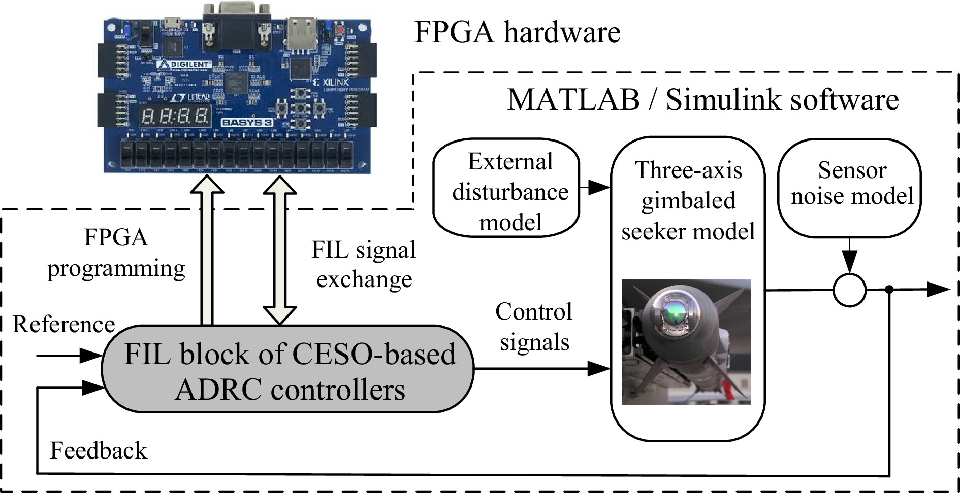
    M. Stanković, S. M. Manojlović, S. M. Simić, S. T. Mitrović, and M. B. Naumović, “FPGA system-level based design of multi-axis ADRC controller,” Mechatronics, vol. 40, pp. 146–155, 2016. doi: 10.1016/j.mechatronics.2016.10.005
  • Related Articles

    [1]Yaozhong Zheng, Hai-Tao Zhang, Ziheng Yu, Xiang Huang, Haichao Jiao, Han Ding. Adaptive Sliding Mode Control with Linear Extended State Observer for Active Magnetic Bearing-Rotor Systems[J]. IEEE/CAA Journal of Automatica Sinica. doi: 10.1109/JAS.2024.125037
    [2]Xiufang Chen, Zhenming Su, Long Jin, Shuai Li. A Correntropy-Based Echo State Network With Application to Time Series Prediction[J]. IEEE/CAA Journal of Automatica Sinica, 2025, 12(2): 425-435. doi: 10.1109/JAS.2024.124932
    [3]Kamal Rsetam, Zhenwei Cao, Zhihong Man, Xian-Ming Zhang. GPIO-Based Continuous Sliding Mode Control for Networked Control Systems Under Communication Delays With Experiments on Servo Motors[J]. IEEE/CAA Journal of Automatica Sinica, 2025, 12(1): 99-113. doi: 10.1109/JAS.2024.124812
    [4]Fazhi Song, Ning Cui, Shuaiqi Chen, Kai Zhang, Yang Liu, Xinkai Chen, Jiubin Tan. Beyond Performance of Learning Control Subject to Uncertainties and Noise: A Frequency-Domain Approach Applied to Wafer Stages[J]. IEEE/CAA Journal of Automatica Sinica, 2025, 12(1): 198-214. doi: 10.1109/JAS.2024.124968
    [5]Qun Lu, Xiang Wu, Jinhua She, Fanghong Guo, Li Yu. Disturbance Rejection for Systems With Uncertainties Based on Fixed-Time Equivalent-Input-Disturbance Approach[J]. IEEE/CAA Journal of Automatica Sinica, 2024, 11(12): 2384-2395. doi: 10.1109/JAS.2024.124650
    [6]Dan Zhang, Jiabin Hu, Jun Cheng, Zheng-Guang Wu, Huaicheng Yan. A Novel Disturbance Observer Based Fixed-Time Sliding Mode Control for Robotic Manipulators With Global Fast Convergence[J]. IEEE/CAA Journal of Automatica Sinica, 2024, 11(3): 661-672. doi: 10.1109/JAS.2023.123948
    [7]Meng Li, Zhigang Zeng. Nested Saturated Control of Uncertain Complex Cascade Systems Using Mixed Saturation Levels[J]. IEEE/CAA Journal of Automatica Sinica, 2024, 11(5): 1163-1174. doi: 10.1109/JAS.2023.124176
    [8]Xiao Xue, Deyu Zhou, Xiangning Yu, Gang Wang, Juanjuan Li, Xia Xie, Lizhen Cui, Fei-Yue Wang. Computational Experiments for Complex Social Systems: Experiment Design and Generative Explanation[J]. IEEE/CAA Journal of Automatica Sinica, 2024, 11(4): 1022-1038. doi: 10.1109/JAS.2024.124221
    [9]Xiao Xue, Xiangning Yu, Deyu Zhou, Xiao Wang, Chongke Bi, Shufang Wang, Fei-Yue Wang. Computational Experiments for Complex Social Systems: Integrated Design of Experiment System[J]. IEEE/CAA Journal of Automatica Sinica, 2024, 11(5): 1175-1189. doi: 10.1109/JAS.2023.123639
    [10]Yunfeng Hu, Chong Zhang, Bo Wang, Jing Zhao, Xun Gong, Jinwu Gao, Hong Chen. Noise-Tolerant ZNN-Based Data-Driven Iterative Learning Control for Discrete Nonaffine Nonlinear MIMO Repetitive Systems[J]. IEEE/CAA Journal of Automatica Sinica, 2024, 11(2): 344-361. doi: 10.1109/JAS.2023.123603
    [11]Zhongcai Zhang, Guangren Duan. Stabilization Controller of An Extended Chained Nonholonomic System With Disturbance:  An FAS Approach[J]. IEEE/CAA Journal of Automatica Sinica, 2024, 11(5): 1262-1273. doi: 10.1109/JAS.2023.124098
    [12]Mengshi Song, Fan Zhang, Bingxiao Huang, Panfeng Huang. Anti-Disturbance Control for Tethered Aircraft System With Deferred Output Constraints[J]. IEEE/CAA Journal of Automatica Sinica, 2023, 10(2): 474-485. doi: 10.1109/JAS.2023.123222
    [13]Lifu Wang, Zhaofei Li, Guotao Zhao, Ge Guo, Zhi Kong. Input Structure Design for Structural Controllability of Complex Networks[J]. IEEE/CAA Journal of Automatica Sinica, 2023, 10(7): 1571-1581. doi: 10.1109/JAS.2023.123504
    [14]Xiufang Chen, Mei Liu, Shuai Li. Echo State Network With Probabilistic Regularization for Time Series Prediction[J]. IEEE/CAA Journal of Automatica Sinica, 2023, 10(8): 1743-1753. doi: 10.1109/JAS.2023.123489
    [15]Jinhua She, Kou Miyamoto, Qing-Long Han, Min Wu, Hiroshi Hashimoto, Qing-Guo Wang. Generalized-Extended-State-Observer and Equivalent-Input-Disturbance Methods for Active Disturbance Rejection: Deep Observation and Comparison[J]. IEEE/CAA Journal of Automatica Sinica, 2023, 10(4): 957-968. doi: 10.1109/JAS.2022.105929
    [16]Haoxiang Ma, Mou Chen, Qingxian Wu. Disturbance Observer-Based Safe Tracking Control for Unmanned Helicopters With Partial State Constraints and Disturbances[J]. IEEE/CAA Journal of Automatica Sinica, 2023, 10(11): 2056-2069. doi: 10.1109/JAS.2022.105938
    [17]Xiao Lu, Linglong Wang, Haixia Wang, Xianghua Wang. Kalman Filtering for Delayed Singular Systems with Multiplicative Noise[J]. IEEE/CAA Journal of Automatica Sinica, 2016, 3(1): 51-58.
    [18]Chaoxu Mu, Qun Zong, Bailing Tian, Wei Xu. Continuous Sliding Mode Controller with Disturbance Observer for Hypersonic Vehicles[J]. IEEE/CAA Journal of Automatica Sinica, 2015, 2(1): 45-55.
    [19]Lu Wang, Jianbo Su. Trajectory Tracking of Vertical Take-off and Landing Unmanned Aerial Vehicles Based on Disturbance Rejection Control[J]. IEEE/CAA Journal of Automatica Sinica, 2015, 2(1): 65-73.
    [20]Wen Qin, Zhongxin Liu, Zengqiang Chen. Formation Control for Nonlinear Multi-agent Systems with Linear Extended State Observer[J]. IEEE/CAA Journal of Automatica Sinica, 2014, 1(2): 171-179.

Catalog

    通讯作者: 陈斌, bchen63@163.com
    • 1. 

      沈阳化工大学材料科学与工程学院 沈阳 110142

    1. 本站搜索
    2. 百度学术搜索
    3. 万方数据库搜索
    4. CNKI搜索

    Figures(9)  / Tables(7)

    Article Metrics

    Article views (127) PDF downloads(33) Cited by()

    /

    DownLoad:  Full-Size Img  PowerPoint
    Return
    Return