A journal of IEEE and CAA , publishes
high-quality papers in English on original
theoretical/experimental research
and development in all areas of automation
 Volume 12
Issue 7
Volume 12
Issue 7
IEEE/CAA Journal of Automatica Sinica
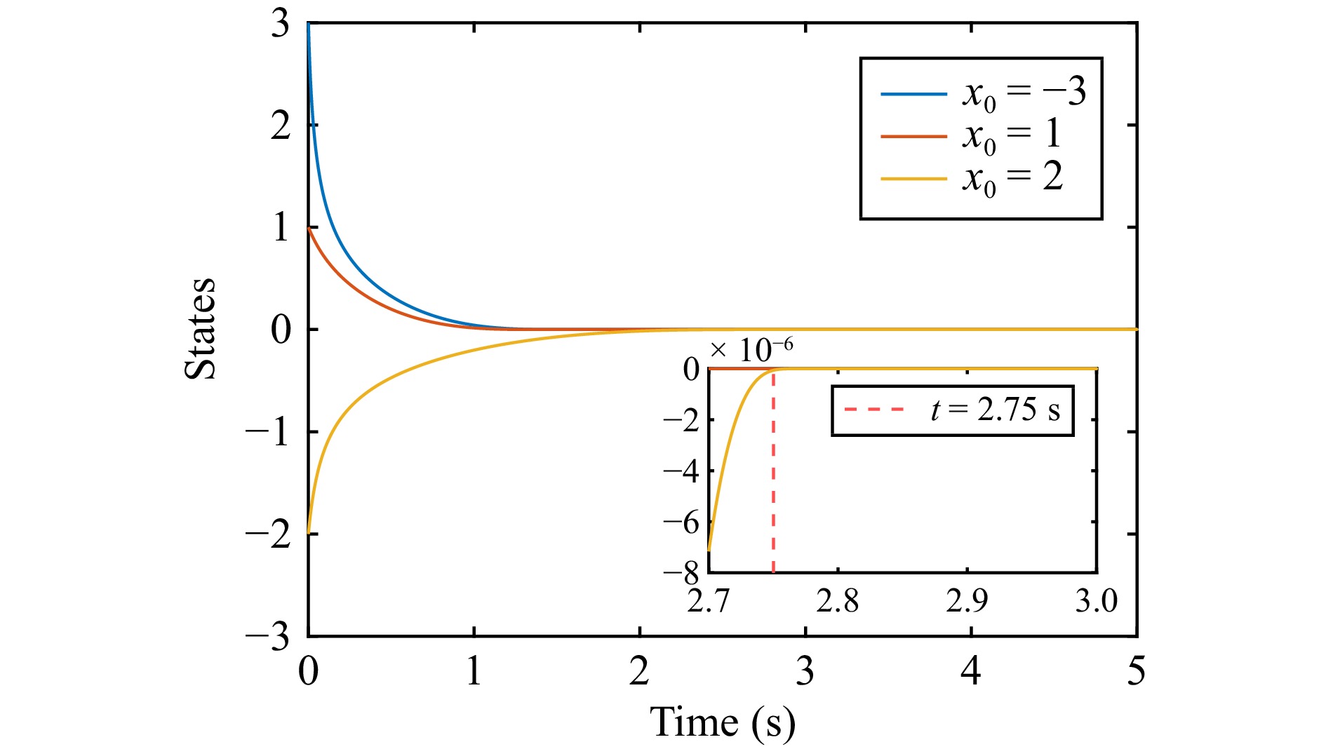
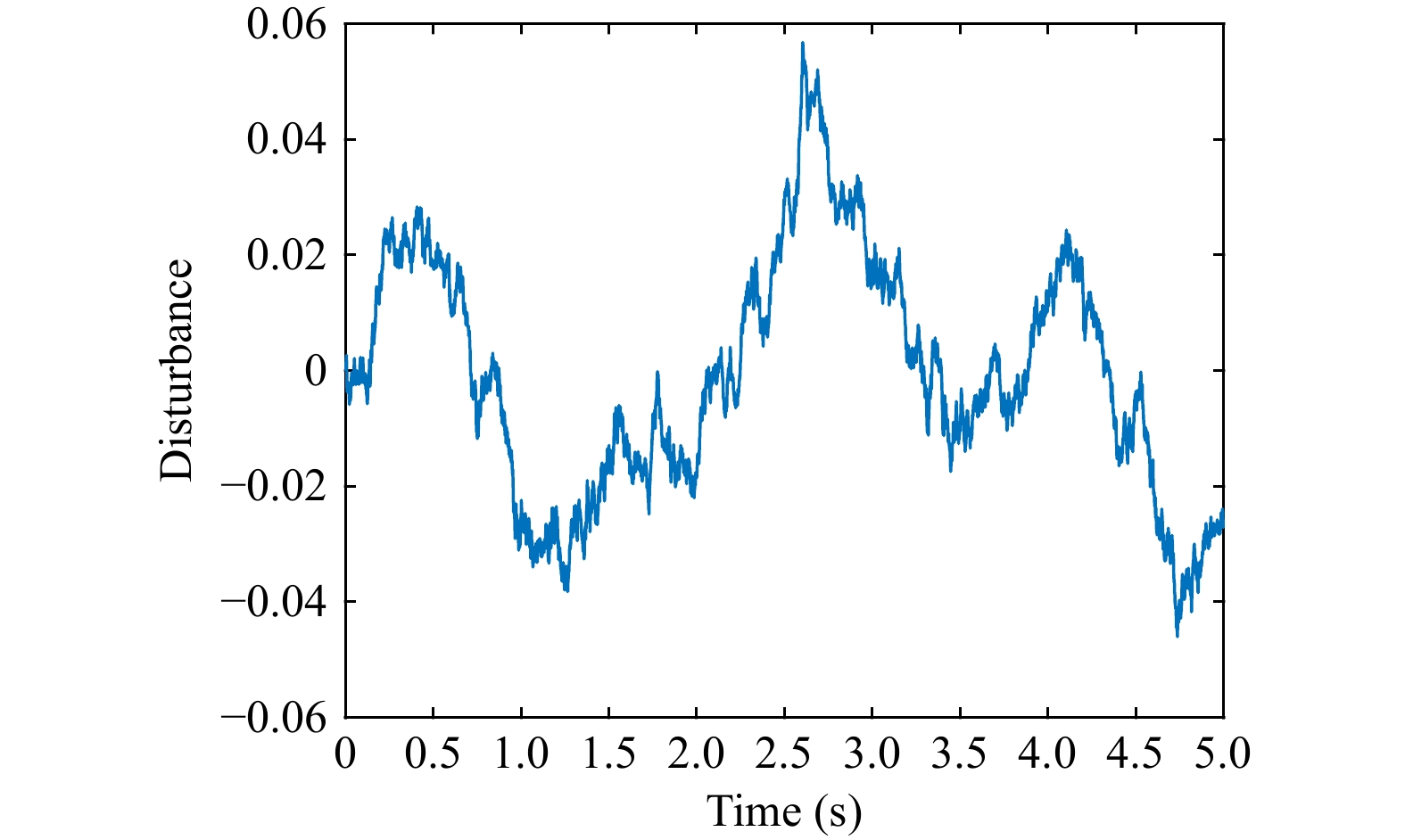
| Citation: | F. Wang, J. Gong, Z. Liu, and F. Chen, “Fixed-time stability of random nonlinear systems,” IEEE/CAA J. Autom. Sinica, vol. 12, no. 7, pp. 1507–1509, Jul. 2025. doi: 10.1109/JAS.2024.124353

|

| [1] |
L. Yao, “Improved stability theorems of random nonlinear time delay systems and their application,” J. Franklin Institute, vol. 359, pp. 5596–5618, 2022. doi: 10.1016/j.jfranklin.2022.05.042
|
| [2] |
M. Cui, L. Geng, and Z. Wu, “Random modeling and control of nonlinear active suspension,” Mathematical Problems in Engineering, vol. 2017, pp. 1–8, 2017.
|
| [3] |
R. Xi, H. Zhang, Q. Liang, and X. Liu, “Command filtered adaptive tracking control for a class of random nonlinear systems,” IEEE Trans. Circuits and Systems II: Express Briefs, vol. 70, pp. 2087–2091, 2023.
|
| [4] |
H. Jian, S. Zheng, P. Shi, Y. Xie, and H. Li, “Consensus for multiple random mechanical systems with applications on robot manipulator,” IEEE Trans. Industrial Electronics, vol. 71, pp. 846–856, 2023.
|
| [5] |
Z. Wu, “Stability criteria of random nonlinear systems and their applications,” IEEE Trans. Autom. Control, vol. 60, no. 4, pp. 1038–1049, 2015. doi: 10.1109/TAC.2014.2365684
|
| [6] |
Z. Wu, H. Karimi, and P. Shi, “Practical trajectory tracking of random Lagrange systems,” Automatica, vol. 105, pp. 314–322, 2019. doi: 10.1016/j.automatica.2019.04.006
|
| [7] |
T. Jiao, W. Zheng, and S. Xu, “Unified stability criteria of random nonlinear time-varying impulsive switched systems,” IEEE Trans. Circuits and Systems I: Regular Papers, vol. 67, no. 9, pp. 3099–3112, 2020. doi: 10.1109/TCSI.2020.2983324
|
| [8] |
R. Wang, H. Wang, W. Li, and B. Niu, “Output tracking control of random nonlinear time-varying systems,” Mathematics, vol. 10, no. 14, p. 2524, 2022.
|
| [9] |
L. Yao and L. Feng, “Noise-to-state finite-time practical stability for random nonlinear systems and its application in random Lagrange systems,” Nonlinear Dynamics, vol. 111, no. 9, pp. 8103–8113, 2023. doi: 10.1007/s11071-023-08261-9
|
| [10] |
H. Li, C. Hua, K. Li, and Q. Li, “Finite-time control of high-order nonlinear random systems using state triggering signals,” IEEE Trans. Circuits and Systems I: Regular Papers, vol. 70, no. 6, pp. 2587–2598, 2023. doi: 10.1109/TCSI.2023.3257868
|
| [11] |
V. Andrieu, L. Praly, and A. Astolfi, “Homogeneous approximation, recursive observer design, and output feedback,” SIAM J. Control and Optimization, vol. 47, no. 4, pp. 1814–1850, 2008. doi: 10.1137/060675861
|
| [12] |
A. Polyakov, “Nonlinear feedback design for fixed-time stabilization of linear control systems,” IEEE Trans. Automatic Control, vol. 57, no. 8, pp. 2106–2110, 2012. doi: 10.1109/TAC.2011.2179869
|
| [13] |
Q. Meng, Q. Ma, and Y. Shi, “Adaptive fixed-time stabilization for a class of uncertain nonlinear systems,” IEEE Trans. Autom. Control, vol. 68, no. 11, pp. 6929–6936, 2023. doi: 10.1109/TAC.2023.3244151
|
| [14] |
B. Zhang, X. Sun, M. Lv, S. Liu, and L. Li, “Distributed adaptive fixed-time fault-tolerant control for multiple 6-DoF UAVs with full-state constraints guarantee,” IEEE Systems J., vol. 16, no. 3, pp. 4792–4803, 2022. doi: 10.1109/JSYST.2021.3128973
|
| [15] |
H. Min, S. Shi, S. Xu, J. Guo, and Z. Zhang, “Fixed-time Lyapunov criteria of stochastic nonlinear systems and its generalization,” IEEE Trans. Autom. Control, vol. 68, no. 8, pp. 5052–5058, 2023. doi: 10.1109/TAC.2022.3218592
|
| [16] |
H. Min, S. Xu, B. Zhang, Q. Ma, and D. Yuan, “Fixed-time Lyapunov criteria and state-feedback controller design for stochastic nonlinear systems,” IEEE/CAA J. Autom. Sinica, vol. 9, no. 6, pp. 1005–1014, 2022. doi: 10.1109/JAS.2022.105539
|
| [17] |
Y. Yang, G. Liu, Q. Li, and C. K. Ahn, “Multiple adaptive fuzzy Nussbaum-type functions design for stochastic nonlinear systems with fixed-time performance,” Fuzzy Sets and Systems, vol. 476, p. 108767, 2024.
|
| [18] |
L. Ren, J. Wu, and J. Liu, “Dynamic event-triggered adaptive fixed-time fuzzy tracking control for stochastic nonlinear systems under asymmetric time-varying state constraints,” Int. J. Fuzzy Systems, vol. 26, no. 1, pp. 73–86, 2024.
|
| [19] |
J. Yin, D. Ding, Z. Liu, and S. Khoo, “Some properties of finite-time stable stochastic nonlinear systems,” Applied Math. and Computation, vol. 259, pp. 686–697, 2015. doi: 10.1016/j.amc.2015.02.088
|
Figures(2)


 DownLoad: