Neural-Network-Based Adaptive Finite-Time Control for a Two-Degree-of-Freedom Helicopter System With an Event-Triggering Mechanism

Zhijia Zhao; Jian Zhang; Shouyan Chen; Wei He; Keum-Shik Hong

doi:10.1109/JAS.2023.123453

Volume 10 Issue 8

Aug. 2023

IEEE/CAA Journal of Automatica Sinica

JCR Impact Factor: 15.3, Top 1 (SCI Q1)

CiteScore: 23.5, Top 2% (Q1)
Google Scholar h5-index: 77， TOP 5

Turn off MathJax

Article Contents

Article Navigation > IEEE/CAA Journal of Automatica Sinica > 2023 > 10(8): 1754-1765

Z. J. Zhao, J. Zhang, S. Y. Chen, W. He, and K.-S. Hong, “Neural-network-based adaptive finite-time control for a two-degree-of-freedom helicopter system with an event-triggering mechanism,” IEEE/CAA J. Autom. Sinica, vol. 10, no. 8, pp. 1754–1765, Aug. 2023. doi: 10.1109/JAS.2023.123453

Citation:

Z. J. Zhao, J. Zhang, S. Y. Chen, W. He, and K.-S. Hong, “Neural-network-based adaptive finite-time control for a two-degree-of-freedom helicopter system with an event-triggering mechanism,” IEEE/CAA J. Autom. Sinica, vol. 10, no. 8, pp. 1754–1765, Aug. 2023. doi: 10.1109/JAS.2023.123453

Citation:

Z. J. Zhao, J. Zhang, S. Y. Chen, W. He, and K.-S. Hong, “Neural-network-based adaptive finite-time control for a two-degree-of-freedom helicopter system with an event-triggering mechanism,” IEEE/CAA J. Autom. Sinica, vol. 10, no. 8, pp. 1754–1765, Aug. 2023. doi: 10.1109/JAS.2023.123453

PDF( 3196 KB)

Neural-Network-Based Adaptive Finite-Time Control for a Two-Degree-of-Freedom Helicopter System With an Event-Triggering Mechanism

doi: 10.1109/JAS.2023.123453

Funds: This work was supported in part by the National Natural Science Foundation of China (62273112, 62061160371, 61933001, 51905115), the Science and Technology Planning Project of Guangzhou City (202201010758), the Guangzhou University-Hong Kong University of Science and Technology Joint Research Collaboration Fund (YH202205), the Open Research Fund from the Guangdong Laboratory of Artificial Intelligence and Digital Economy (Shenzhen (SZ)) (GML-KF-22-27), and the Korea Institute of Energy Technology Evaluation and Planning Through the Auspices of the Ministry of Trade, Industry and Energy, Republic of Korea (20213030020160)

More Information

Author Bio:
Zhijia Zhao (Member, IEEE) received the B.Eng. degree in automatic control from North China University of Water Resources and Electric Power in 2010, and the M.Eng. and Ph.D. degrees in automatic control from South China University of Technology, in 2013 and 2017, respectively.He is currently an Associate Professor at the School of Mechanical and Electrical Engineering, Guangzhou University. His research interests include adaptive and learning control, flexible mechanical systems, and robotics

Jian Zhang received the B.Eng. degree from West Anhui University in 2020. He is currently pursuing the master degree at the School of Mechanical and Electrical Engineering, Guangzhou University.His research interests include adaptive control, intelligent control, and robotics

Shouyan Chen received the B.Eng. degree in process control and the Ph.D. degree in mechanical design from the South China University of Technology, in 2008 and 2017, respectively.He is currently an Associate Professor at the School of Mechanical and Electrical Engineering, Guangzhou University. His research interests include robotics, human-robot interaction, and intelligent control

Wei He (Senior Member, IEEE) received the B.Eng. and the M.Eng. degrees from the College of Automation Science and Engineering, South China University of Technology, in 2006 and 2008, respectively, and the Ph.D. degree from the Department of Electrical and Computer Engineering, the National University of Singapore, Singapore, in 2011. He is now working as a Full Professor at the School of Intelligence Science and Technology, University of Science and Technology Beijing. He has co-authored 3 books published in Springer and published over 100 international journal and conference papers. He was awarded a Newton Advanced Fellowship from the Royal Society, UK in 2017. He was a recipient of the IEEE SMC Society Andrew P. Sage Best Transactions Paper Award in 2017. He is serving the Chair of IEEE SMC Society Beijing Capital Region Chapter. From 2018, he has been the Chair of Technical Committee on Autonomous Bionic Robotic Aircraft, IEEE Systems, Man and Cybernetics Society. He has been serving as an Associate Editor/Guest Editor of several prestigious scientific journals, including IEEE Transactions on Robotics, IEEE Transactions on Neural Networks and Learning Systems, IEEE Transactions on Control Systems Technology, IEEE Transactions on Systems, Man, and Cybernetics: Systems, SCIENCE CHINA Information Sciences, IEEE/CAA Journal of Automatica Sinica, Neurocomputing, and an Editor of Journal of Intelligent and Robotic Systems. His research interests extend to robotics, distributed parameter systems, and intelligent control systems

Keum-Shik Hong (Fellow, IEEE) received the B.S. degree in mechanical design from Seoul National University, Korea (south) in 1979, the M.S. degree in mechanical engineering from Columbia University, USA, in 1987, and both the M.S. degree in applied mathematics and the Ph.D. degree in mechanical engineering from the University of Illinois at Urbana-Champaign, USA in 1991. He joined the School of Mechanical Engineering, Pusan National University, Korea (south) in 1993.He served as Associate Editor of Automatica (2000–2006), as Editor-in-Chief of the Journal of Mechanical Science and Technology (2008–2011), and is serving as the Editor-in-Chief of the International Journal of Control, Automation, and Systems. He was a past President of the Institute of Control, Robotics and Systems (ICROS), Korea, and is President of the Asian Control Association. He is an IEEE Fellow, a Fellow of the Korean Academy of Science and Technology, an ICROS Fellow, and a Member of the National Academy of Engineering of Korea. He has received many awards, including the Best Paper Award from the KFSTS of Korea (1999) and the Presidential Award of Korea (2007). His research interests include brain-computer interface, nonlinear systems theory, adaptive control, and distributed parameter systems
Corresponding author: Zhijia Zhao, e-mail: zhjzhaoscut@163.com; Shouyan Chen, e-mail: maxcsy@gzhu.edu.cn
Received Date: 2022-12-29
Accepted Date: 2023-01-26

Available Online: 2023-04-18

Abstract

Abstract

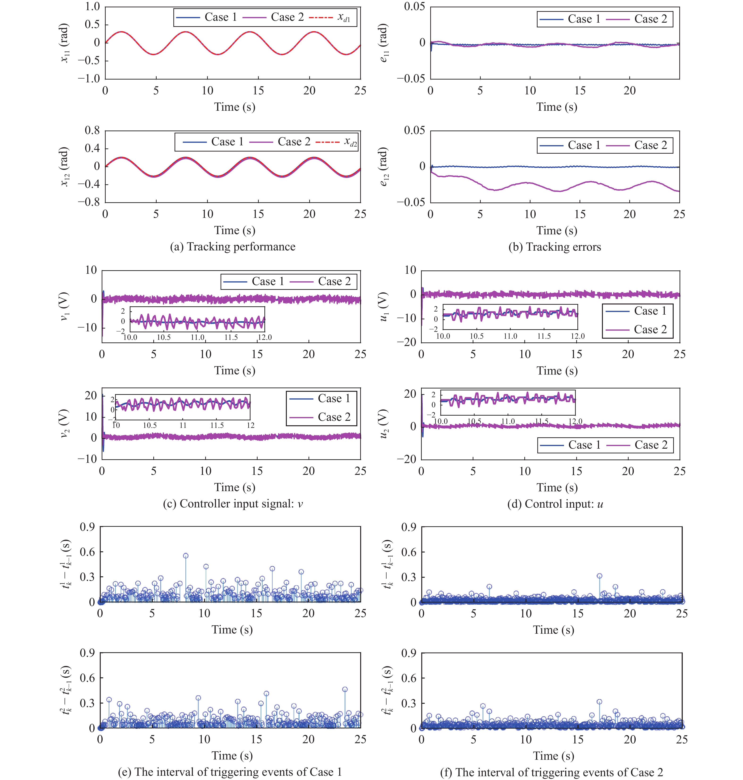
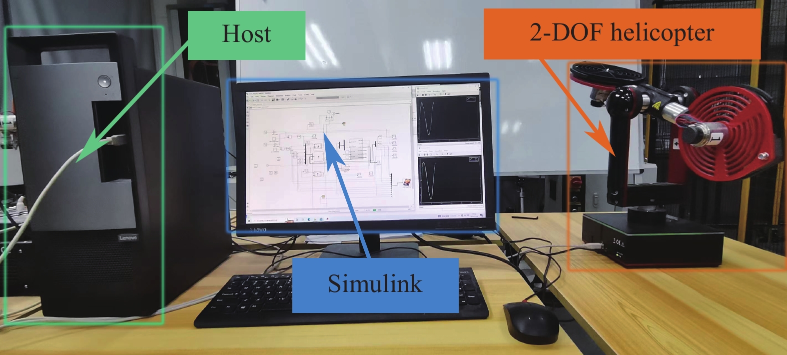
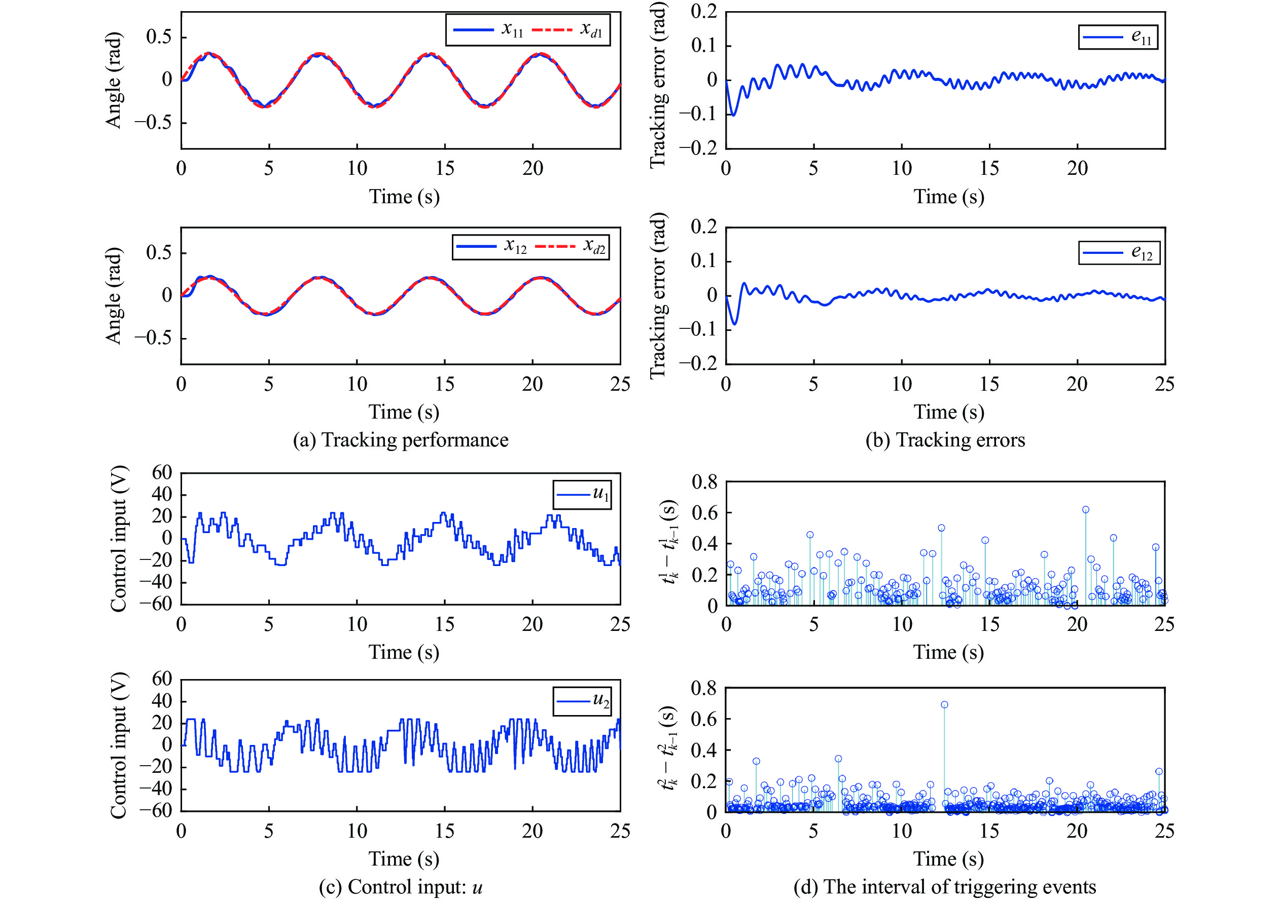
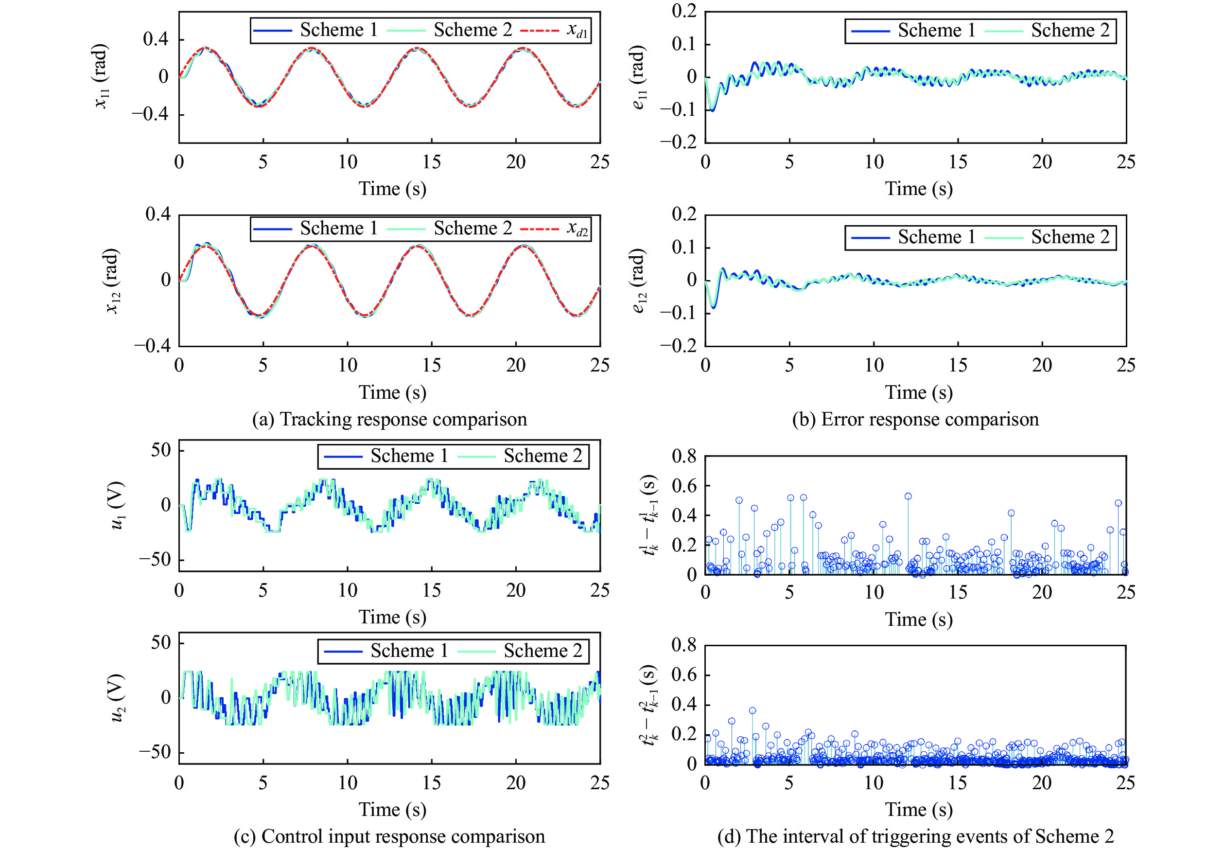
Helicopter systems present numerous benefits over fixed-wing aircraft in several fields of application. Developing control schemes for improving the tracking accuracy of such systems is crucial. This paper proposes a neural-network (NN)-based adaptive finite-time control for a two-degree-of-freedom helicopter system. In particular, a radial basis function NN is adopted to solve uncertainty in the helicopter system. Furthermore, an event-triggering mechanism (ETM) with a switching threshold is proposed to alleviate the communication burden on the system. By proposing an adaptive parameter, a bounded estimation, and a smooth function approach, the effect of network measurement errors is effectively compensated for while simultaneously avoiding the Zeno phenomenon. Additionally, the developed adaptive finite-time control technique based on an NN guarantees finite-time convergence of the tracking error, thus enhancing the control accuracy of the system. In addition, the Lyapunov direct method demonstrates that the closed-loop system is semiglobally finite-time stable. Finally, simulation and experimental results show the effectiveness of the control strategy.
- Adaptive neural-network control,
- event-triggering mechanism (ETM),
- finite time,
- two-degree-of-freedom helicopter

FullText(HTML)

References(38)

References

[1]	S.-K. Kim, K. S. Kim, and C. K. Ahn, “Order reduction approach to velocity sensorless performance recovery PD-type attitude stabilizer for 2-DOF helicopter applications,” IEEE Trans. Industrial Informatics, vol. 18, no. 10, pp. 6848–6856, 2022. doi: 10.1109/TII.2022.3143204
[2]	M. Chen, P. Shi, and C.-C. Lim, “Adaptive neural fault-tolerant control of a 3-DOF model helicopter system,” IEEE Trans. Systems,Man,and Cybernetics: Systems, vol. 46, no. 2, pp. 260–270, 2016. doi: 10.1109/TSMC.2015.2426140
[3]	R. Singh and B. Bhushan, “Data-driven technique-based fault-tolerant control for pitch and yaw motion in unmanned helicopters,” IEEE Trans. Instrumentation and Measurement, 2020, DOI: 10.1109/TIM.2020.3025656.
[4]	S.-K. Kim and C. K. Ahn, “Performance-boosting attitude control for 2-DOF helicopter applications via surface stabilization approach,” IEEE Trans. Industrial Electronics, vol. 69, no. 7, pp. 7234–7243, 2022. doi: 10.1109/TIE.2021.3095799
[5]	B. Zheng and Y. Zhong, “Robust attitude regulation of a 3-DOF helicopter benchmark: Theory and experiments,” IEEE Trans. Industrial Electronics, vol. 58, no. 2, pp. 660–670, 2011. doi: 10.1109/TIE.2010.2046579
[6]	C. K. Verginis, C. P. Bechlioulis, A. G. Soldatos, and D. Tsipianitis, “Robust trajectory tracking control for uncertain 3-DOF helicopters with prescribed performance,” IEEE/ASME Trans. Mechatronics, 2021, DOI: 10.1109/TMECH.2021.3136046.
[7]	C. Zhu, Y. Jiang, and C. Yang, “Fixed-time neural control of robot manipulator with global stability and guaranteed transient performance,” IEEE Trans. Industrial Electronics, vol. 70, no. 1, pp. 803–812, 2023. doi: 10.1109/TIE.2022.3156037
[8]	Z. Zhao, W. He, C. Mu, T. Zou, K.-S. Hong, and H.-X. Li, “Reinforcement learning control for a 2-DOF helicopter with state constraints: Theory and experiments,” IEEE Trans. Automation Science and Engineering, DOI: 10.1109/TASE.2022.3215738.
[9]	Z. Zhao, W. He, J. Yang, and Z. Li, “Adaptive neural network control of an uncertain 2-DOF helicopter system with input backlash and output constraints,” Neural Computing and Applications, vol. 34, no. 20, pp. 18143–18154, 2022. doi: 10.1007/s00521-022-07463-3
[10]	J. Zhang, Y. Yang, Z. Zhao, and K. S. Hong, “Adaptive neural network control of a 2-DOF helicopter system with input saturation,” Int. J. Control,Autom. and Systems, vol. 21, no. 1, pp. 318–327, 2023. doi: 10.1007/s12555-021-1011-2
[11]	S. Shao and M. Chen, “Adaptive neural discrete-time fractional-order control for a uav system with prescribed performance using disturbance observer,” IEEE Trans. Systems,Man,and Cybernetics: Systems, vol. 51, no. 2, pp. 742–754, 2021. doi: 10.1109/TSMC.2018.2882153
[12]	Z. Liu, J. Shi, Y. He, Z. Zhao, and H.-K. Lam, “Adaptive fuzzy control for a spatial flexible hose system with dynamic event-triggered mechanism,” IEEE Trans. Aerospace and Electronic Systems, DOI: 10.1109/TAES.2022.3197551.
[13]	X. Guo, D. Zhang, J. Wang, and C. K. Ahn, “Adaptive memory event-triggered observer-based control for nonlinear multi-agent systems under DoS attacks,” IEEE/CAA J. Autom. Sinica, vol. 8, no. 10, pp. 1644–1656, 2021. doi: 10.1109/JAS.2021.1004132
[14]	L. Liu, X. Li, Y. J. Liu, and S. Tong, “Neural network based adaptive event trigger control for a class of electromagnetic suspension systems,” Control Engineering Practice, vol. 106, 2021.
[15]	Z. Wu, J. Xiong, and M. Xie, “A switching method to event-triggered output feedback control for unmanned aerial vehicles over cognitive radio networks,” IEEE Trans. Systems,Man,and Cybernetics: Systems, vol. 51, no. 12, pp. 7530–7541, 2021. doi: 10.1109/TSMC.2020.2971726
[16]	L. Dou, S. Cai, X. Zhang, X. Su, and R. Zhang, “Event-triggered-based adaptive dynamic programming for distributed formation control of multi-UAV,” J. the Franklin Institute, vol. 359, no. 8, pp. 3671–3691, 2022. doi: 10.1016/j.jfranklin.2022.02.034
[17]	H. Liang, X. Guo, Y. Pan, and T. Huang, “Event-triggered fuzzy bipartite tracking control for network systems based on distributed reduced-order observers,” IEEE Trans. Fuzzy Systems, vol. 29, no. 6, pp. 1601–1614, 2021. doi: 10.1109/TFUZZ.2020.2982618
[18]	X. Zhao, S. Zhang, Z. Liu, J. Wang, and H. Gao, “Adaptive event-triggered boundary control for a flexible manipulator with input quantization,” IEEE/ASME Trans. Mechatronics, pp. 1–11, 2021.
[19]	H. Pan, D. Zhang, W. Sun, and X. Yu, “Event-triggered adaptive asymptotic tracking control of uncertain mimo nonlinear systems with actuator faults,” IEEE Trans. Cybernetics, vol. 52, no. 9, pp. 8655–8667, 2022. doi: 10.1109/TCYB.2021.3061888
[20]	Z. Zhao and Z. Liu, “Finite-time convergence disturbance rejection control for a flexible timoshenko manipulator,” IEEE/CAA J. Autom. Sinica, vol. 8, no. 1, pp. 157–168, 2021. doi: 10.1109/JAS.2020.1003378
[21]	H. Wang, W. Bai, and X. Liu, “Finite-time adaptive fault-tolerant control for nonlinear systems with multiple faults,” IEEE/CAA J. Autom. Sinica, vol. 6, no. 6, pp. 1417–1427, 2019. doi: 10.1109/JAS.2019.1911765
[22]	L. Kong, Q. Lai, Y. Ouyang, Q. Li, and S. Zhang, “Neural learning control of a robotic manipulator with finite-time convergence in the presence of unknown backlash-like hysteresis,” IEEE Trans. Systems,Man,and Cybernetics: Systems, vol. 52, no. 3, pp. 1916–1927, 2022. doi: 10.1109/TSMC.2020.3034757
[23]	Q. Chen, Y. Ye, Z. Hu, J. Na, and S. Wang, “Finite-time approximation-free attitude control of quadrotors: Theory and experiments,” IEEE Trans. Aerospace and Electronic Systems, vol. 57, no. 3, pp. 1780–1792, 2021. doi: 10.1109/TAES.2021.3050647
[24]	W. Yang, G. Cui, Z. Li, and C. Tao, “Fuzzy approximation-based adaptive finite-time tracking control for a quadrotor UAV with actuator faults,” Int. Journal of Fuzzy Systems, DOI: 10.1007/s40815-022-01361-5.
[25]	J. Sun, J. Yi, and Z. Pu, “Fixed-time adaptive fuzzy control for uncertain nonstrict-feedback systems with time-varying constraints and input saturations,” IEEE Trans. Fuzzy Systems, vol. 30, no. 4, pp. 1114–1128, 2022. doi: 10.1109/TFUZZ.2021.3052610
[26]	Y. Li, Y.-X. Li, and S. Tong, “Event-based finite-time control for nonlinear multi-agent systems with asymptotic tracking,” IEEE Trans. Automatic Control, pp. 1–8, DOI: 10.1109/TAC.2022.3197562.
[27]	C.-H. Zhang and G.-H. Yang, “Event-triggered global finite-time control for a class of uncertain nonlinear systems,” IEEE Trans. Automatic Control, vol. 65, no. 3, pp. 1340–1347, 2020. doi: 10.1109/TAC.2019.2928767
[28]	J. Sun, H. He, J. Yi, and Z. Pu, “Finite-time command-filtered composite adaptive neural control of uncertain nonlinear systems,” IEEE Trans. Cybernetics, vol. 52, no. 7, pp. 6809–6821, 2022. doi: 10.1109/TCYB.2020.3032096
[29]	Q. Inc., “Quanser aero laboratory guide,” Technical Report, Quanser, 2016.
[30]	T. Zou, H. Y. Wu, W. Sun, and Z. Zhao, “Adaptive neural network sliding mode control of a nonlinear two-degrees-of-freedom helicopter system,” Asian J. Control, DOI: 10.1002/asjc.2862.
[31]	M. Chen and G. Tao, “Adaptive fault-tolerant control of uncertain nonlinear large-scale systems with unknown dead zone,” IEEE Trans. Cybernetics, vol. 46, no. 8, pp. 1851–1862, 2016. doi: 10.1109/TCYB.2015.2456028
[32]	S. Li, L. Ding, H. Gao, Y.-J. Liu, L. Huang, and Z. Deng, “Adaptive fuzzy finite-time tracking control for nonstrict full states constrained nonlinear system with coupled dead-zone input,” IEEE Trans. Cybernetics, vol. 52, no. 2, pp. 1138–1149, 2022. doi: 10.1109/TCYB.2020.2985221
[33]	C. Wang, Y. Li, Q. Hu, and J. Huang, “Event-triggered adaptive control for attitude tracking of spacecraft,” Chinese J. Aeronautics, vol. 32, no. 2, pp. 454–462, 2019. doi: 10.1016/j.cja.2018.12.021
[34]	H. Wang, C. Bing, and L. Chong, “Adaptive neural control for strict-feedback stochastic nonlinear systems with time-delay,” Neurocomputing, vol. 77, no. 1, pp. 267–274, 2012. doi: 10.1016/j.neucom.2011.08.020
[35]	X. Wang, D. Ding, H. Dong, and X.-M. Zhang, “Neural-network-based control for discrete-time nonlinear systems with input saturation under stochastic communication protocol,” IEEE/CAA J. Autom. Sinica, vol. 8, no. 4, pp. 766–778, 2021. doi: 10.1109/JAS.2021.1003922
[36]	Z. Zhang, C. Wen, L. Xing, and Y. Song, “Adaptive event-triggered control of uncertain nonlinear systems using intermittent output only,” IEEE Trans. Autom. Control, vol. 67, no. 8, pp. 4218–4225, 2022. doi: 10.1109/TAC.2021.3115435
[37]	X. Wang, D. Ding, X. Ge, and Q.-L. Han, “Neural-network-based control for discrete-time nonlinear systems with denial-of-service attack: The adaptive event-triggered case,” Int. J. Robust and Nonlinear Control, vol. 32, no. 5, pp. 2760–2779, 2022. doi: 10.1002/rnc.5831
[38]	X. Wang, D. Ding, X. Ge, and Q.-L. Han, “Supplementary control for quantized discrete-time nonlinear systems under goal representation heuristic dynamic programming,” IEEE Trans. Neural Networks and Learning Systems, pp. 1–13, DOI: 10.1109/TNNLS.2022.3201521.

Supplements(0)

Cited By

Proportional views

Proportional views

通讯作者: 陈斌, bchen63@163.com

1.
沈阳化工大学材料科学与工程学院沈阳 110142

Figures(7) / Tables(1)

Get Citation

PDF

XML

Article Metrics

Article views (514) PDF downloads(162)

Highlights

A new event triggering mechanism (ETM) for greater flexibility and save communication resources
Utilize ETM to save system communication resources while considering finite time convergence
It ensures that the closed-loop signal of the system is half-leaf finite time stable

Neural-Network-Based Adaptive Finite-Time Control for a Two-Degree-of-Freedom Helicopter System With an Event-Triggering Mechanism

doi: 10.1109/JAS.2023.123453

Abstract

References

Proportional views

Catalog

通讯作者: 陈斌, bchen63@163.com

Article Metrics

Highlights

Export File

Citation

Format

Content