A journal of IEEE and CAA , publishes
high-quality papers in English on original
theoretical/experimental research
and development in all areas of automation
C. H. Liu, F. Zhu, Q. Liu, and Y. C. Fu, "Hierarchical Reinforcement Learning With Automatic Sub-Goal Identification," IEEE/CAA J. Autom. Sinica, vol. 8, no. 10, pp. 1686-1696, Oct. 2021. doi: 10.1109/JAS.2021.1004141
Citation:
C. H. Liu, F. Zhu, Q. Liu, and Y. C. Fu, "Hierarchical Reinforcement Learning With Automatic Sub-Goal Identification," IEEE/CAA J. Autom. Sinica, vol. 8, no. 10, pp. 1686-1696, Oct. 2021. doi: 10.1109/JAS.2021.1004141
C. H. Liu, F. Zhu, Q. Liu, and Y. C. Fu, "Hierarchical Reinforcement Learning With Automatic Sub-Goal Identification," IEEE/CAA J. Autom. Sinica, vol. 8, no. 10, pp. 1686-1696, Oct. 2021. doi: 10.1109/JAS.2021.1004141
Citation:
C. H. Liu, F. Zhu, Q. Liu, and Y. C. Fu, "Hierarchical Reinforcement Learning With Automatic Sub-Goal Identification," IEEE/CAA J. Autom. Sinica, vol. 8, no. 10, pp. 1686-1696, Oct. 2021. doi: 10.1109/JAS.2021.1004141
School of Computer Science and Technology, Soochow University, Suzhou 215006, China
2.
School of Computer Science and Engineering, Changshu Institute of Technology, Changshu 215500, China
Funds:
This work was supported by the National Natural Science Foundation of China (61303108), Suzhou Key Industries Technological Innovation-Prospective Applied Research Project (SYG201804), A Project Funded by the Priority Academic Program Development of Jiangsu Higher Education Institutions (PAPD), and the Fundamental Research Funds for the Gentral Universities, JLU (93K172020K25)
Chenghao Liu is a postgraduate of School of Computer Science and Technology, Soochow University. His main research interests include reinforcement learning, deep reinforcement learning, and hierarchical reinforcement lerning
Fei Zhu is Ph.D. and Associate Professor in School of Computer Science and Technology, Soochow University. He is a Member of China Computer Federation. His main research interests include deep learning, reinforcement learning, text mining, and pattern recognition. He studies to design and applies machine learning algorithms to solve health data science, health informatics, predictive analytics, and personalized data-driven decision support problems
Quan Liu is Ph.D. and Professor in School of Computer Science and Technology, Soochow University. His main research interests include intelligence information processing, automated reasoning, and machine learning
Yuchen Fu is Ph.D. and Professor in School of Computer Science and Engineering, Changshu Institute of Technology. His main research interests include reinforcement learning, intelligence information processing, and machine learning. He was Chairman of Suzhou Sub-Forum Academic Committee of CCF YOCSEF, Executive Member of Suzhou Division of China Computer Federation
In reinforcement learning an agent may explore ineffectively when dealing with sparse reward tasks where finding a reward point is difficult. To solve the problem, we propose an algorithm called hierarchical deep reinforcement learning with automatic sub-goal identification via computer vision (HADS) which takes advantage of hierarchical reinforcement learning to alleviate the sparse reward problem and improve efficiency of exploration by utilizing a sub-goal mechanism. HADS uses a computer vision method to identify sub-goals automatically for hierarchical deep reinforcement learning. Due to the fact that not all sub-goal points are reachable, a mechanism is proposed to remove unreachable sub-goal points so as to further improve the performance of the algorithm. HADS involves contour recognition to identify sub-goals from the state image where some salient states in the state image may be recognized as sub-goals, while those that are not will be removed based on prior knowledge. Our experiments verified the effect of the algorithm.
DEEP reinforcement learning, controlled by input information, similar to the decision mode of humans, is a combination of deep learning and reinforcement learning [1]. Since Manih et al. introduced the deep Q network (DQN) [2], applications of deep reinforcement learning have continued to increase and many improved DQN algorithms have been proposed, such as double Q-learning [3], the Priority Replay Buffer [4] and the Dueling Deep Q Network (DuDQN) [5], which solve the control problem in the continuous action space with a human-level performance.
However, these algorithms perform poorly in tasks with sparse rewards, e.g., the Montezuma game where agents barely find reward points. In order to solve these problems, hierarchical reinforcement learning is used to deal with such problems, such as with the abstract method proposed by Sutton et al. [6], where abstraction was used to decompose large-scale problems into smaller ones and complex problems into simpler ones. After the agent solves all the decomposed problems, the complex large problem is then correspondingly resolved. Hierarchical deep reinforcement learning, which takes advantage of the concept of hierarchy in deep reinforcement learning, consists of hierarchical reinforcement learning and deep learning. Kulkarni et al. proposed hierarchical deep reinforcement learning (hDQN) [7], which alleviates the sparse reward problem by constructing hierarchical decision models and setting up small goals. Andrychowicz et al. proposed hindsight experience replay (HER) [8], which made the agents’ learning relatively smooth by establishing relatively feasible goals. Florensa et al. introduced a stochastic network for hierarchical reinforcement learning [9], which divided tasks into two layers and learned useful skills in a pretrained environment. Le et al. put forth hierarchical imitation reinforcement learning to solve the problem of sparse rewards by imitating the behavior of human experts [10].
In hierarchical deep reinforcement learning, sub-goal identification is a crucial issue, where a well chosen sub-goal speeds up learning [11]. Methods to find sub-goals in hierarchical reinforcement learning include determining sub-goals based on the state access frequency, recognizing sub-goals based on the state transition graph or common subspace, etc. Rafati and Noelleproposed a model-free algorithm for detecting sub-goals associated with the intrinsic motivation learning mechanism, learning sub-goals and skills based on the experience from the environment [12]. Imani and Braga-Neto used a partially observable boolean dynamic system (POBDS) signal model to measure the time sequence of noise expression in Boolean GRN and developed the Bayes inverse reinforcement learning (BIRL) [13]. Dilokthanakul et al. proposed an algorithm with the advantage of learning representations from intrinsic rewards to improve the performance of HER [14]. However, the majority of approaches require defining sub-goals manually, which not only causes poor performance in complex problems, but also results in poor generalization ability, difficulty in determining sub-goals in large space, and large deviations between manual methods and other methods.
To address the problem, we propose a hierarchical deep reinforcement learning algorithm with automatic sub-goal identification via computer vision (HADS), which obtains the sub-goals from pixels. One of the goals of automatic control of hierarchical deep reinforcement learning is to detect sub-goals without any human intervention. However it is very hard to achieve at present. Standard approaches for detecting sub-goals require heavy computation while the performance is not as good as expected. Some points are in fact unreachable, such as points behind the walls, as well as fringe points. As for obstacles, if they are identified as sub-goal points, the agent gets a positive reward when reaching these points, while according to most settings the agent gets a negative reward, which is a contradiction. Correspondingly, obstacle points are also removed. Removing these points helps to improve the performance. Although our ultimate goals are to provide automatic control, it is worth adding a little bit of human knowledge to enhance behavior of the algorithm. The paper is organized as follows. In Section II, we introduce preliminaries, including reinforcement learning, hierarchical reinforcement learning and hierarchical deep reinforcement learning. In Section III, we expand the model and the processing workflow of the HADS algorithm. In Section IV, we explain the experiments and analyze the results of experiment. In Section V, we conclude our work.
II.
Preliminaries
A
Reinforcement Learning
Reinforcement learning, which is different from supervised learning and unsupervised learning, is a trial-and-error method in which the agent receives a reward signal in exploration process rather than receiving timely feedback [15]. Reinforcement learning consists of four elements, including the state, action, reward, and environment, where for the environment, the agent interacts with it to obtain a higher reward; the state refers to the single state in the state space that the agent is in for each time step; the action refers to the single action in the action space that the agent adopts for each time step; the reward refers to the reward the agent receives for adopting a certain action.
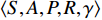
A reinforcement learning problem can be modelled with a Markov decision process (MDP) by a tuple ⟨S,A,P,R,γ⟩ where S is a state set, A is an action set, P is the state transition probability, R is a reward function, and γ∈[0,1] is a discount factor. A policy π is a distribution over actions given states, π(a|s)=P[At=a|St=s]. Q-learning [16], a classical algorithm of reinforcement learning, where temporal-difference (TD) [1] is utilized, uses a Q value to evaluate the action under some certain state. Q(st,at), the expected cumulative reward of taking action at in state st, is calculated as follows:
δ=Rt+1+γmaxaQ(st+1,a)−Q(st,at)
(1)
Q(st,at)=Q(st,at)+αδ
(2)
where α is the step size parameter, Rt+1 is the immediate reward and γ is the discount rate. In this case, the Q-value function that is near the optimal state action-value function is denoted as Q∗.
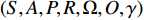
The partially observable Markov decision process (POMDP) is a variation of MDP in which the POMDP model only has part of the information. POMDP is represented by a tuple (S,A,P,R,Ω,O,γ), where Ω is a group of result sets which contain the environment data collected by the sensor, and O is the situation-observation probability, that is, the probability the agent is under state s when it observes the environment data o. In POMDP, since the information is inadequate, the history sequence information is utilized to estimate the state, referred to as the belief state.
Recently, deep reinforcement learning (DRL), which combines deep learning with reinforcement learning, has achieved much success. Deep reinforcement learning algorithms usually learn control strategies from high-dimensional raw data directly. In particular, as a widely used deep reinforcement learning algorithm, DQN takes advantage of a convolutional neural network (CNN) [17] to get state information from pixel data and makes a decision by using Q-learning.
B
Hierarchical Reinforcement Learning
Hierarchical reinforcement learning is an extended framework of common reinforcement learning [18], e.g., HAM [19], Options [20], MAXQ [21], and HER [8], which decompose the original tasks into smaller and simpler sub-tasks so as to form a hierarchical structure. Learning tasks are assigned to each sub-task, which, according to reinforcement learning methods, explores policy in the constrained task hierarchical space [22]. As soon as the policy exploration of each sub-task is completed, the policy of the original task is also achieved.
Abstraction [20] is a key issue in hierarchical reinforcement learning, by which some irrelevant or redundant information from different sub-tasks are removed so as to simplify the problem. There are various abstractions in hierarchical reinforcement learning, including state abstraction (space abstraction) [23], task abstraction [24], and time abstraction (action abstraction) [25]. Space abstraction can be divided into two cases: one is to encapsulate several states so as to form a single abstract state; the other is to simplify the state representation by deleting state variables independent of sub-states in the case of a decomposable state. Task abstraction decomposes the main learning task into several sub-tasks by some evaluation index, solves the sub-tasks separately by which the whole problem can be solved. Time abstraction encapsulates several actions as a single abstract action, of which the purpose is to make full use of the hierarchical structure of the problem. Each abstract action corresponds to a closed-loop local policy defined on a subset of environmental states with termination conditions, which is called Option or Temporally-extended actions that is a framework based on time abstraction [20].
Abstract action is an important concept in the Option framework, which uses prior knowledge to speed up learning. It is known that the reuse of a learned model can speed up learning. In practice, it is of very little value to have two tasks that are exactly the same. Therefore, it is usually unable to achieve reuse at the entire task level. In fact, it is more likely that two tasks are partially similar, making it is possible to apply reuse at a more subtle level, i.e., to reuse policy of subtasks rather than the entire task. Although the sharing policy of the sub-task has many constraints, it really provides a feasible way for the present. The abstract action includes the basic action defined in the corresponding problem domain. A reinforcement learning agent can select an abstract action in a certain state and then execute the abstract action according to the policy, until the termination condition is satisfied.
C
DRL With Time Abstraction
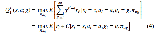
The difference between deep reinforcement learning with time abstraction [26] and standard deep reinforcement learning is that deep reinforcement learning with time abstraction appends a goal g to Q value. The corresponding Q estimates of the controller are
where g is the goal at state s, πag is the policy currently adopted, and E represents expectation. The Q estimates of the meta-controller are also derived from the previously aforementioned equations
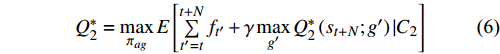
C2=st=s,gt=g,πag
(5)
Q∗2=maxπagE[t+N∑t′=tft′+γmaxg′Q∗2(st+N;g′)|C2]
(6)
where N is the time steps required for the controller to achieve its goal, g′ represents the agent’s goal at st+N, and πg is the policy adopted by the meta-controller to reach the goal g [27].
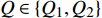
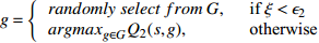
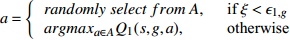
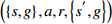
In DQN, the Q value is constantly updated to approach the optimal [28] value, and the Q value with target g can also be expressed by adding parameter θ:Q∗(s;g)≈Q(s,g;θ). Similar but different from DQN, each Q∈{Q1,Q2} needs to be trained to minimize loss functions L1(θ1) and L2(θ2) [29]. The interaction sequences (st,gt,ft,st+N) of Q2 and (st,at,gt,rt,st+1) are stored in corresponding replay buffers D1 and D2. The loss function of Q value is defined as mean squared error. The loss function of Q1 is similar to that of DQN.
L1(θ1,i)=E(s,a,g,r,s′D1)[(y1,i−Q1(s,a;θ1,i,g))2]
(7)
y1,i=r+γmaxa′Q1(s′,a′;θ1,i−1,g)
(8)
where i represents the number of iterations, y1,i is determined by (8), and E represents expectation. When the loss function is updated during the optimization stage, the parameters of the previous iterations, θ1,i−1 remain unchanged. The gradient is used to optimize the parameter θ1.
R=r+γmaxa′Q1(s′,a′;θ1,i−1,g)
(9)
τ=R−Q1(s,a;θ1,g)
(10)
▽θ1,iL1(θ1,i)=Es,a,g,r,s′D1[τ▽θ1,iQ1(s,a;θ1,g)].
(11)
Loss function L2 and its gradient updating parameters [30] can also be obtained in the same way.
D
Improving Exploration by Sub-Goal Identification
Exploration and exploitation are important issues in reinforcement learning [31], in which, given a single policy agent, during exploration, one tries to find a larger search space so as to get a better policy, bringing a higher cost but not necessarily a higher success rate; during exploitation, the agent adopts the optimal policy with the highest estimated reward at present. Performing too much exploration requires lots of computation despite the fact that it provides a higher probability of attaining a better global or near-optimum solution; although excessive exploitation speeds up convergence, it often leads to a local optimum. The efficiency of an algorithm lies on the fine balance of exploration and exploitation [32].
In a Markov process, effective exploration is indispensable to learn a better control policy [33], which, is a major challenge. Although some methods have been proposed, searching for more effective exploration methods has been an ongoing direction in reinforcement learning. In the study of reinforcement learning, the most frequently used policy is ϵ−greedy, which plays an important role in common reinforcement learning, because it chooses the best policy for the time being, taking into account the exploration to prevent falling into a local optima. However, due to the sparsity of rewards and the large state space, common methods often fail to find out the final goal [34].
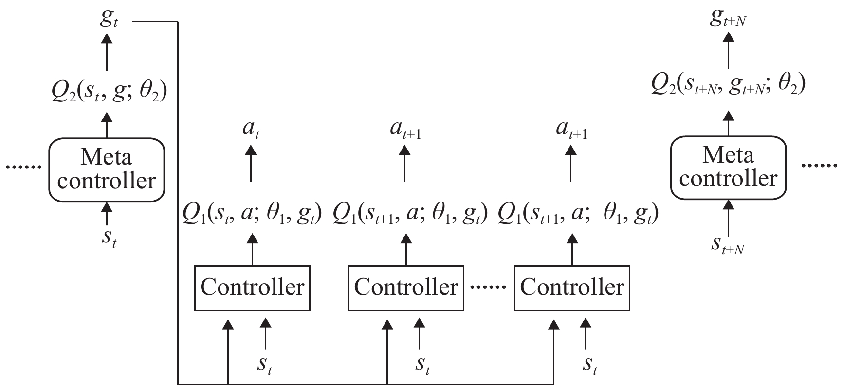
By exploring a series of internal goals set in advance, the agent achieves the goal during which it is necessary to learn the corresponding policy for that goal. An internal reward [35] is used to determine whether the agent has reached the goal point, and to optimize the corresponding policy. In deep hierarchical reinforcement learning, Kulkarni et al. [7] proposed a framework for deep hierarchical learning (hDQN), where agents adopted a two-layer hierarchical structure, which was composed of the meta-controller and the controller. The meta-controller interacts with the environment to get the state st, and then chooses a goal gt∈G, where G is the current set of all possible goals.
After the meta-controller chooses the goal gt, the controller chooses the action at according to the current state st and gt. It requires certain time steps for the agent to reach gt or the final state. As shown in Fig. 1 [7], the meta-controller chooses a goal gt, and in the next period, the controller tries to reach gt. In the framework of hDQN, there is an internal critic module [36], which verifies whether the controller has reached the corresponding goal gt and returns an appropriate internal reward rt(g) to the controller. If the controller reaches the corresponding goal, it gets a reward of 1 or a reward of 0 otherwise. The goal of the controller is to maximize the cumulative internal rewards, Rt(g)=∑∞t′=tγt′−trt(g). Similarly, the goal of the meta-controller is to maximize the cumulative external rewards, Ft=∑∞t′=tγt′−tft′, where ft′ is the cumulative reward for interaction with the external environment in time step t, where ft′ are the rewards after finishing a series of sub-goals.
Figure
1.
Meta-controller selects the goal g, and the controller completes the goal g. The meta-controller selects a sub-goal g that is supposed to visited by controller. At state st, the sub-goal gt is generated by the meta-controller for the controller. The controller gets to gt after N steps. The procedure will be carried on iteratively with the task is completed
As soon as the sub-goals are completed, the agent can successfully reach the end point, and be rewarded. In order to let the agent reach the sub-goal with a better method, the controller is optimized by incorporating the internal reward function, so the agent can reach the sub-goal quickly and finally reach the end point smoothly.
III.
Algorithm Description
On the basis of the original hDQN algorithm, the function of automatic sub-goal identification is incorporated, which makes the original hierarchical reinforcement learning algorithm more intelligent by identifying sub-goals from the image. By capturing states from the state image, the algorithm searches for the sub-goals, and improves them to so that they are higher quality by taking advantage of prior knowledge. Then the sub-goals and the image are put into a neural network to be trained together. As there are some sub-goals that are unreachable, we need to incorporate criteria to tailor original sub-goals. First, as the fringe parts are unreachable, the fringe sub-goal points should be filtered; second, as for obstacle points, the agent will receive a negative reward when reaching obstacles, and will receive a positive one when reaching a sub-goal, which is a contradiction; third, some sub-goal points that are helpless to the mission are filtered.
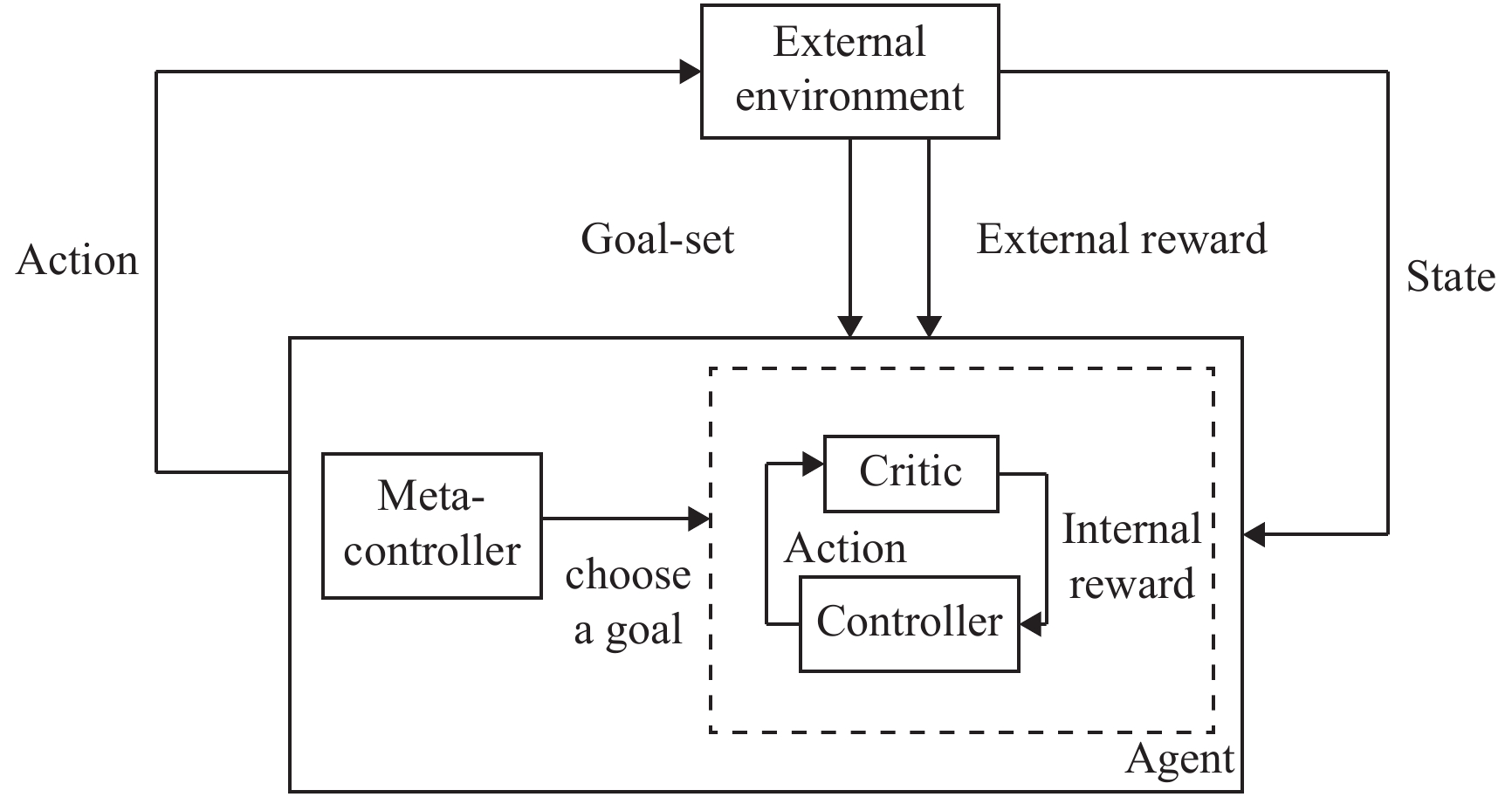
Fig. 2 shows the illustration of the interaction between the agent and environment, where the environment provides the reward as well as a sub-goal set. When the controller achieves the target, an internal reward is provided by the critic. The environment generates a set of sub-goals for the meta-controller according to its understanding of the environment from Fig. 3. The agent receives the current state, the meta-controller chooses the goal according to the received state, and the controller generates the action according to the received state and the selected goal. Once the controller reaches the goal chosen by the meta-controller, the critic will give the controller a positive internal reward. Otherwise, if the goal is not reached, the reward given by the critic is 0, and the reward given by the external environment is negative. The final goal of the meta-controller is the end point that the agent needs to reach. The controller achieves the last goal when the agent reaches the end point.
Figure
2.
In the model framework, for the interaction between the agent and environment, the environment provides not only the outer reward but also a sub-goal set. When the controller achieves the target (as stated previously), an internal reward is provided by the critic part
Figure
3.
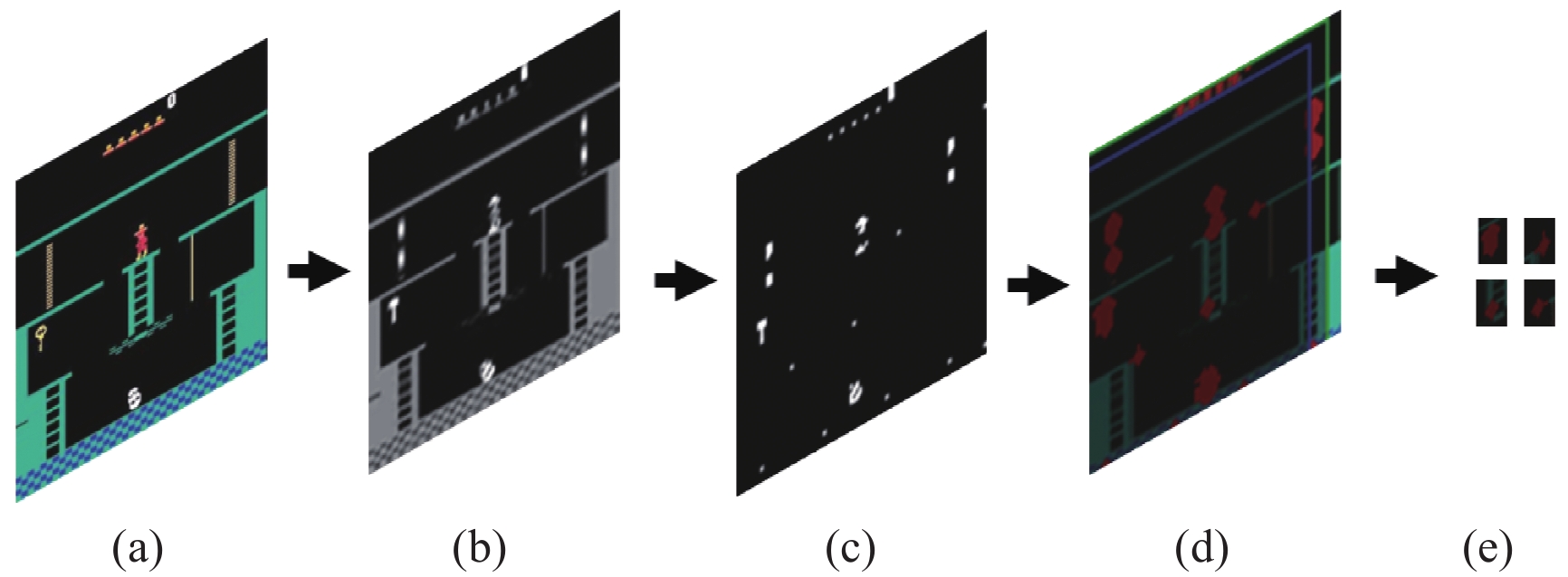
The generation of sub-goals where (a) represents the raw image as the input; (b) represents the gray-scale image from the raw image; (c) represents the binary image from the gray-scale image; (d) represents the detected sub-goal based on (c); and (e) represents the processed sub-goal points
Like most standard deep reinforcement learning algorithms, our method takes images as initial input to extract sub-goals. The state image needs to be processed at first because the original image contains much redundant information. Preserving valuable pixels, the image is cut to the fixed size because the network requires pictures of uniform size. After obtaining the image, we adopt a method in which the two-dimensional Gauss template is used to perform smoothing filtering to remove the noise of the image. The smaller scale template is used to ensure the accuracy of locating the contour of the object in the image on a large scale, which will blur the edge of the contour of the object and affect the subsequent detection. Then the smoothed image is processed using object edge detection, and the preliminary response image is obtained [37]. At this time, a blurred location of the contour of the object’s edge has been obtained, and the final step is to locate it accurately. The non-maximum suppression method is used to refine the image processed above, in which only the points with the greatest local variation are retained, and the edge image of the single-pixel object is obtained. According to the binary image, after the contour position of the object is obtained, the coordinates are obtained.
There are several coordinates obtained, each corresponding to a set of coordinates, but the sub-goal points used in deep learning are not a group, for which a set of coordinates need to be processed. However, there are still two problems concerning the obtained target points. The first problem is that the coordinates of the target points are a group rather than a single point, and the data types are not consistent with the ones used in the algorithm. The second problem is that these target points are not necessarily what we need. Therefore, in order to solve the problem of a set of coordinates in the algorithm, the average value of the set of coordinates is taken as its corresponding sub-goal points. For the data type problem, the obtained goal points are converted into data types compatible with the network without changing their original meanings. On the basis of prior knowledge, some sub-goal points which can not be explored by an agent as well as some meaningless sub-goal points are removed to ensure that the obtained goal points are reachable and meaningful. For example, in snapshots of game controlling, part of the image represents the life value of agents, which is unimportant to an agent. In the exploration process, there exists some places that are beyond the reach of agents, and thus would be regraded as meaningless points, and be removed from sub-goals. In addition, according to the initial position of the agent in the game, we rank the distance from the target point to the initial position of the agent. Let the agent explore these sub-goal points from the near ones to the distant ones in the initial stage of exploration, which is equivalent to providing a relatively good policy for the agent at the beginning. However, the algorithm still uses the ϵ−greedy policy to explore, utilizing the provided policy to attempt to achieve better result.
The size of the adjusted image is 84×84×1 or 84×84×3 and the former is more easily processed. We use the standard method to process gray-scale maps so as to convert the image to a Gray map by GRAYmap=0.3×R+0.59×G+0.11×B where R is red, G is green, and B is blue. In Algorithm 1 the image is processed to obtain sub-goals where the input image for the training network is raw RGB images. We utilize findContours in OpenCV to get the contour that is needed in the experiment from the binary-value image.
Algorithm 1 Automatic Discovery of Sub-Goal
Require: state image
Ensure: sub-goal set G
1: Cut the state image to 84 × 84 × 1, and get R, G, and B value of each pixel
2: Convert original image into gray image by:
GRAYmap=0.3×R+0.59×G+0.11×B
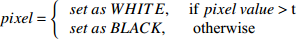
3: Calculate the average pixel of an image as a threshold t
7: Detect external contour to get a set of coordinates of target points G1={g11,..,g1n,g21,...,g2n,...,gnn} by using function findContours
8: Turn a set of coordinates corresponding to each goal point into G2={g′1,g′2,...,g′n}
9: Data type consistency processing G2={g1″ with data used in subsequent algorithms
10: for each g in G_{2} do
11: ifg is fringe or obstacle or miscellaneous then
12: remove g
13: else
14: reserve g
15: end if
16: end for
17: Put all reserved g into G=\left\{ g_{1},g_{2},...,g_{m} \right\}
B
Hierarchical Deep Reinforcement Learning With Sub-Goals
The obtained sub-goals are applied to hierarchical deep reinforcement learning described, as follows.
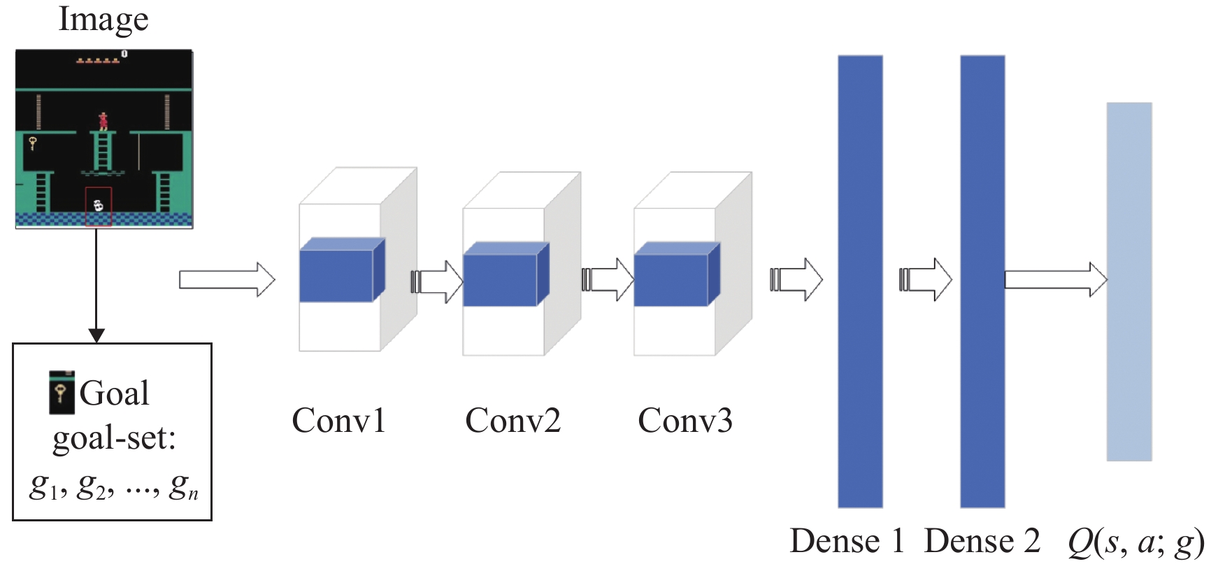
The algorithm uses dual network structures, which are different from the standard network structure in that our algorithm has sub-goal points. The corresponding network structure of the controller is to store samples with goal points in the corresponding replay buffer at each time step. The network structure corresponding to the meta-controller is that when the goal selected by the meta-controller is completed, the samples obtained by the meta-controller are stored in the replay buffer corresponding to the meta-controller. In this way, a hierarchical structure is constructed. The network structure corresponding to the controller is shown as Fig. 4. The network structure corresponding to the meta-controller is similar to that of Fig. 4. Since the framework in this paper is based on Deep Reinforcement Learning, the complexity of the framework is equivalent with that of the framework decided by the numbers of convolution layers and full-connected layers. Like DQN network structure, our proposed network contains 3 convolutional layers and 2 full-connected layers, solving more complex problems (the input includes sub-goals) at the cost of higher expenses. The time complexity of DQN is approximately O(E\times B\times T), where E represents the number of plots, B represents the batch size, and T represents the time complexity of the network. On the basis of DQN, our algorithm adds the process of finding sub-goals. Since the time complexity of finding sub-goals algorithm is O(n) , the time complexity of our algorithm is approximately O(E\times B\times T)+O(n).
Figure
4.
Diagram of network structure where the image and sub-goal set are taken as the input of the network of 3 hidden layers and 2 fully connected layers with the output being a Q value with the sub-goal g
There are lots of studies on deep reinforcement learning. The DQN algorithm is a benchmark approach of deep reinforcement learning; the DuDQN algorithm is an improved algorithm based on the DQN algorithm; the hDQN algorithm is based on hierarchical reinforcement learning with a neural network for solving large-scale continuous problems. We compared performance of our proposed algorithms with DQN, DuDQN, and hDQN. In some areas, although manually selecting sub-goals does bring a better result, it depends on human efforts and has too many constraints. In discrete areas there are various approaches for automatically searching sub-goals but in continuous areas there are no such approaches. Thus, we used the Computer Vision approach to search for sub-goals. But because of the complexity of the environment, it still requires a little manual intervention.
A
Montezuma’s Revenge
As is shown in Fig. 5, in Montezuma’s Revenge, the agent needs to find the key and use it to open the door. The agent will get a reward when it gets the key, and another reward when it gets the key and opens the door. This is characterized by features of sparse reward problems. Therefore, in order to simplify the problem, without changing the final solution, the agent is regarded as completing the task when it gets a reward. In this game, we altered the reward criteria used by DQN and other algorithms with the reward being assigned 0 for failure and 1 for succeeding in executing sub-goals. The reward setting does not essentially change the problem, and better demonstrates the result. In the experiments, we stipulate that the reward is 0 for each step of the agent, –1 for failure, or 5 for getting the external reward. Since the rewards are sparsely distributed, in most cases the agent can not find the reward points; if the reward is not altered, the result often appears to be a horizontal line, inconvenient for analysis. The learning rate is 0.00025 and the discount factor is 0.99. Although there are many tools, such as AutoML [38], that enable the agent to automatically tune hyper-parameters so as to get better performance, we did not take advantage of them in order to evaluate approaches in a fair way, because we need to use the same hyper-parameter settings used in Kulkarni et al. [7].
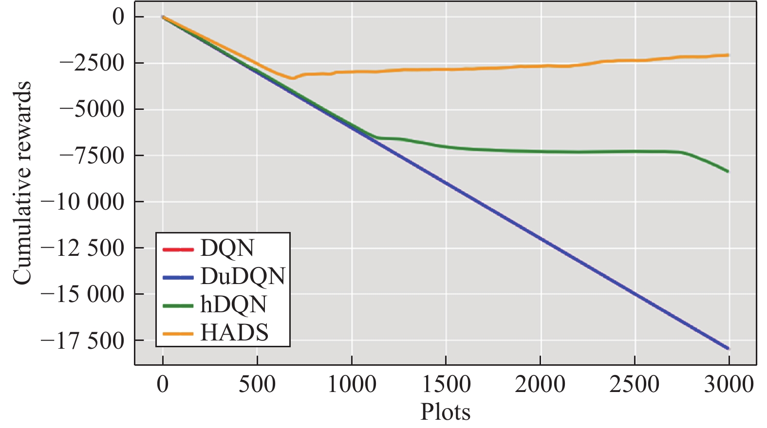
The sub-goal is obtained by Algorithm 1, which is shown in red dot in Fig. 6(a), where it can be seen that, when the unreachable sub-goal points are not removed, the number of original sub-goal points is too large. If agents explore based on these sub-goal points, the performance of the algorithm cannot be improved. Therefore, according to some prior knowledge, we need to remove those points, such as the number of life values on the top of the graph and the agent itself. The number of life values that is used to indicate the remaining number of lives of the agent can not be explored. Similarly, some other unexplored points are also removed, and the resulting figure is shown in Fig. 6(b), where the sub-goal points are much less than those in the top graph, and they are all accessible sub-goal points. Some reachable sub-goal points are helpless to the mission and are also filtered, such as the door.
Figure
6.
Original generated sub-goal graph and sub-goal graph after removing unreachable sub-goal points. In (a), the blurred red dots are initial sub-goal points, with some of them being unattainable for the agent and some of them being non-real sub-goal points, that is, on the agent itself. In (b), the red rectangle marks the actual sub-goal points
As is shown in Fig. 6(b), in the middle of the agent and the ladder on the right, we find the sub-goal point, that is, the first sub-goal point explored by the agent which will be much faster than the first sub-goal point explored by the hDQN. The sub-goal points found in HADS are a little more than those manually identified sub-goal points. It is undeniable that the manually defined sub-goal points are very important, but adding some sub-goal points between these important sub-goal points can improve the speed of reaching these important sub-goal points.
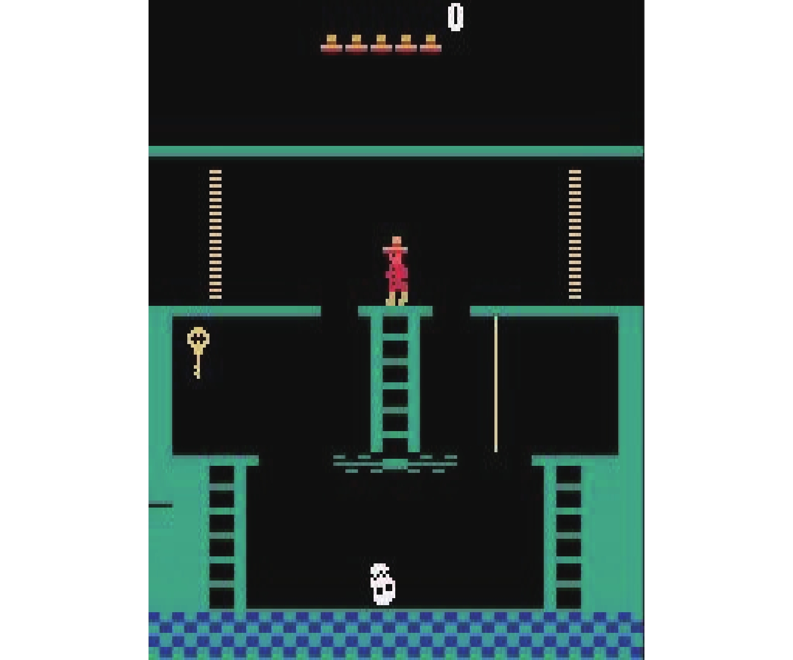
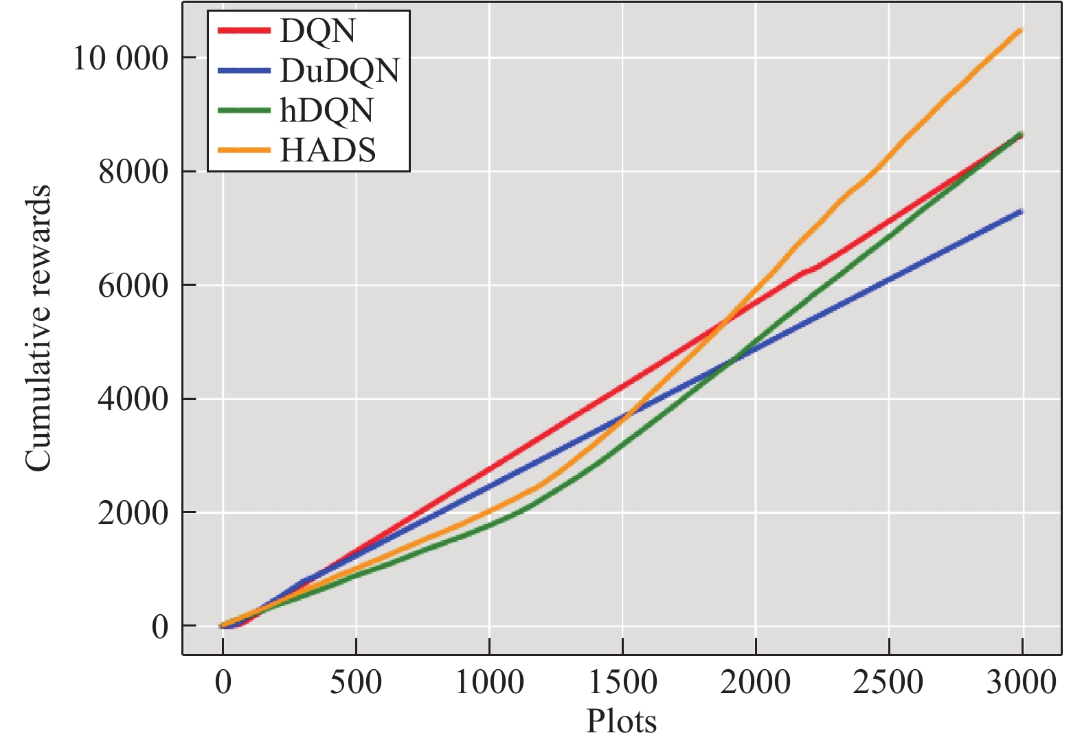
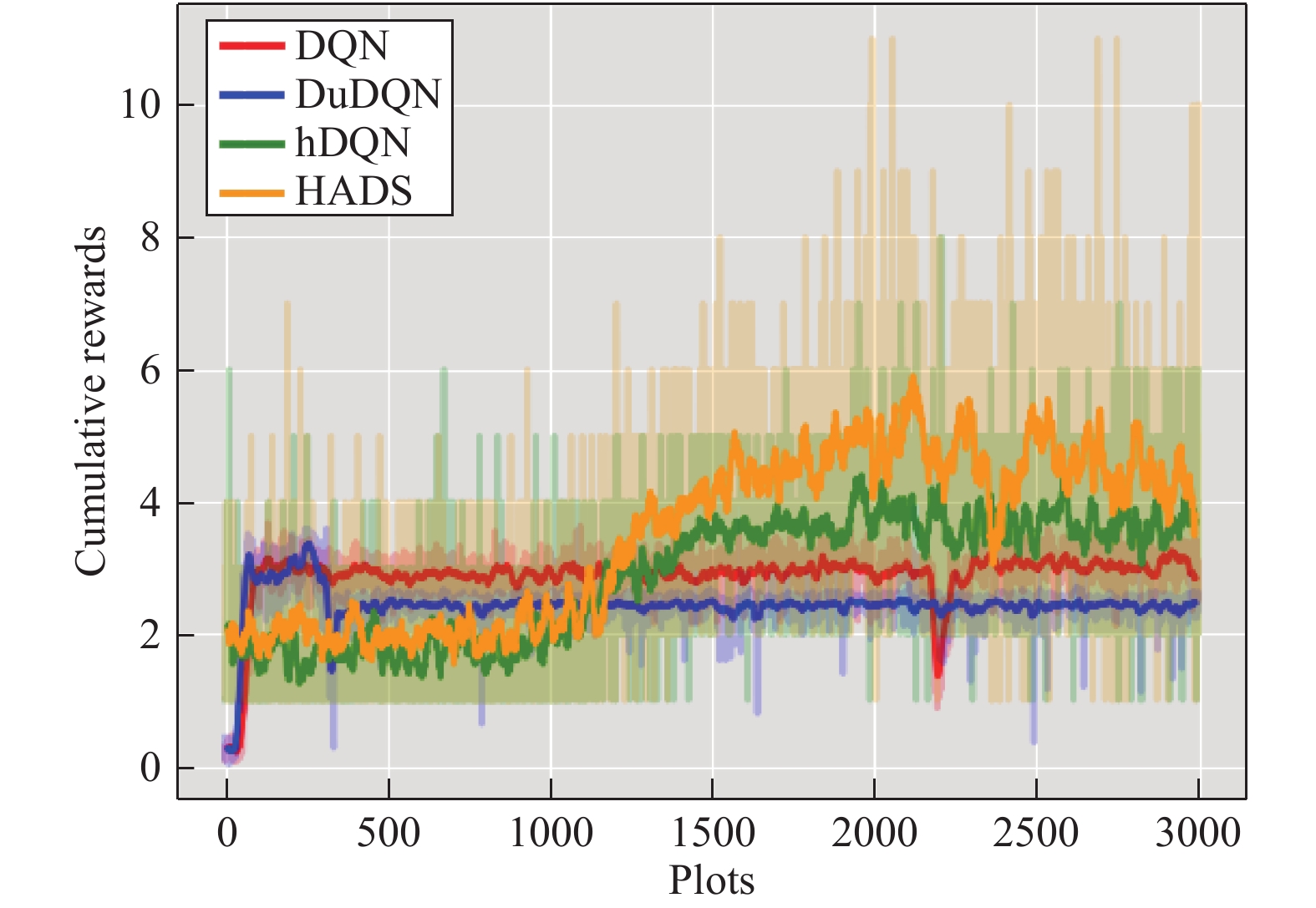
The number of plots of the experiment is set as 3000 and the maximum number of steps per plot is set as 5000. In a plot, if the agent takes 5000 steps and is still alive, or if the agent does not find a reward point, the plot ends. Similarly, the experiment also sets up 20 000 steps for the agent to explore randomly. In these 20 000 steps, the network is not used to train. At the end of the random exploration, we began to use the network to train, and finally obtain the cumulative reward of all plots as shown in Fig. 7, the reward of each plot returned is shown in Fig. 8, and the average reward of the 3000 plot is shown in Table I.
Figure
7.
Cumulative external rewards. The result trend of DQN overlapped with that of DuDQN. HADS got a better convergence rate, as it has more sub-goals than hDQN
Figure
8.
Reward for each plot. HADS is better than the other three approaches, because sub-goals alleviated the sparse problem which made DQN and DuDQN incapable of solving the task
Table I demonstrates that the average rewards of hDQN and HADS for the 3000th plot are superior to those of DQN and DuDQN. Fig. 7 indicates that DQN has not explored the reward point in the searching process until the end of the plot, and each time the value of life is used up, no reward point is found. It can be seen from the Figs. 7 and 8, that the result trend of DQN overlapped with that of DuDQN. These two algorithms do not explore reward points. However, in the original data, it is found that DuDQN still has reward points, although very few. In hDQN, the three manually defined sub-goal points are the right ladder, the left ladder and the key in Fig. 5, sequentially, and the three points are set with increasingly internal rewards. The hDQN performed much better than DQN, and DuDQN, while HADS surpassed hDQN, as can be seen from Table II, where we listed the average value (Avg), maximum value (max), minimum value (min), and mean square deviation (MSD). Since Fig. 7 is a graph of cumulative rewards, the trend of each algorithm is shown. Because we do not know if there are significant differences between these values, we draw the mean value chart and various tables for comparison and the MSD value is also given in the tables. Because DQN and DuDQN do not get rewards in the current environment, the MSD value of both algorithms is 0. The reason why HADS is slightly higher than hDQN is that the sub-goal points in hDQN are given manually, so hdqn will be slightly lower than HADS.
As can be seen from Fig. 8, before 700 plots, hDQN and HADS received almost the same reward for each plot, and after 700 plots, the reward for each plot of HADS was higher than that of hDQN, which shows that HADS had an advantage over hDQN, DQN, and DuDQN. From Table III, we can see that although our proposed algorithm, HADS, was not as good as an expert player, it really achieved automatic control and, more importantly, showed a better trend. We believe that with more subtle training, HADS could attain even better results. In Fig. 8, the dotted line is the real reward for each plot, while the solid line is the average reward for 30 episodes. Therefore, according to the effect in the figure, HADS shows the best experimental effect.
Table
III.
Results With Expert Player for 30 Plots
Kangaroo is also a strategy game, which aims to find rewarding points. Unlike in Montezuma’s Revenge, in Kangaroo the reward is not sparse, which makes it a bit different from reward setting in Montezuma’s Revenge: if the reward point is found, the reward point will be set to 1; otherwise, if the agent fails, the reward is set to 0. An illustration of Kangaroo is shown in Fig. 9.
In the experiment, the sub-goals are obtained by algorithm 1 first. Kangaroo’s original sub-goals are highlighted in the red dot in Fig. 10(a). If the original unreachable sub-goal points are unchanged, it is more difficult to improve performance as there are many sub-goal points which requires much computational cost. Since some goal points are not explored by the agent, it is logical to eliminate them. Therefore, according to prior knowledge, some points were removed, such as the staircase-like object on the left side, the number of life values, and the score attained in the bottom. As can be seen, the sub-goal points are much less than those in left-hand graph, and they are all accessible sub-goal points.
Figure
10.
Original generated sub-goal graph and sub-goal graph after removing unreachable sub-goal points. In (a), the blurred red dots are initial sub-goal points, with some of them being unattainable for the agent and some of them being not real sub-goal points, that is, being on the agent itself. In (b), the red rectangle denotes the actual sub-goal points
The experiment takes 3000 plots, where the maximum number of steps for each plot is 5000, i.e., if an agent survives 5000 steps in a plot, or if the agent has not explored the reward point, the plot will end. Similarly, the experiment sets up 20 000 steps for algorithms to explore randomly. The algorithms do not start training the network until the end of the exploration stage. Finally, a cumulative reward for all the plots is recorded, as shown in Fig. 11, a reward for each plot as shown in Fig. 12, and an average reward for the 3000 plots as shown in Table IV.
Figure
11.
Kangaroo cumulative external rewards. DQN was the most stable. DuDQN did not achieve a better result. After 1300 plots, hDQN and HADS got better results than DQN. Finally the maximum reward of the HADS was better than the other three algorithms
Figure
12.
Kangaroo reward for each plot. DQN and DuDQN have more stable trend. HADS and hDQN have better results. Before the 1200 plots, because Options have not been constructed, hDQN and HADS did not perform well. However, after successfully setting up Options, HADS and hDQN showed a powerful capacity and got much better results
As can be seen from Table IV, the average rewards of hDQN and HADS for the 3000th plot are better than those of DQN and DuDQN. From Fig. 11, we can see that DQN performs well, making progress steadily. Although DuDQN is also growing better, it is not as good as DQN in terms of training results. The improvement of DuDQN over DQN is not decisive in Kangaroo. hDQN did not perform well in earlier stage because hDQN needs two networks to be trained, which requires more time and samples. After training for a certain plots, the strong growth rate of hDQN proved its strength. HADS has a similar result to that of hDQN. Compared with hDQN, the HADS algorithm pays much attention to automatic discovery of sub-goals. In the process of sub-goal identification, only a few manual intervention was incorporated during sub-goal detection, the sub-goal identified by HADS are better than the sub-goals automatically defined by hDQN, and Fig. 11 demonstrates that the final result is better than that of hDQN algorithm. As shown in Fig. 11, the sub-goals identification by HADS are superior to those automatically defined by hDQN. Therefore, on this basis, the effect of HADS is naturally better than that of hDQN. As can be seen from Table V, we show the average value, maximum, minimum and mean square deviation. Fig. 11 is similar to Fig. 7.
It can be seen that DQN and hDQN are relatively stable, but the rewards in each plot are relatively low. The rewards of hDQN and HADS are not stable. But after 1000 plots, the rewards of the two algorithms begin to grow and soon exceed the rewards of DQN, and the rewards of HADS are the highest. As can be seen from Fig. 12, the performance of HADS is better than that of hDQN because of the sub-goals found. The expert player has obvious advantages over other algorithms, because the expert player has significant experience. After training, our algorithms also get a better training result.
C
t-Test
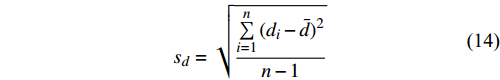
In this section, we utilize the paired sample t-test to evaluate the difference between average results of the experiments. The t-test includes the single population test and double population test, where the single population t-test is used to test whether the difference between the average of a sample and that of a known population is significant. The double population t-test can be divided into two situations: one is an independent sample t-test, which is used to test the difference of the data obtained by two groups of unrelated samples; the other is a paired sample t-test, which is used to test the difference between the data obtained by two groups of subjects or the data obtained by the same group of subjects under different conditions. The samples following two situations are the relevant samples. We used the method of the paired sample test, and the equations [39] for obtaining t-value is as follows:
\begin{array}{l} t = \dfrac{\bar{d}-\mu_0 }{s_d/\sqrt{n}} \end{array} \qquad\qquad
where \bar{d} is the average of paired sample differences, s_d is the standard deviation of paired sample difference, n is the number of paired samples, n - 1 is the degrees of freedom and \mu_0 is the average value of original sample. According to the number of samples and the table of t-bounds, the p-value corresponding to t-value can be obtained to judge whether the difference between the two results is significant.
DQN and DuDQN suffer from sparse problem. As a result, by using DQN and DuDQN to solve the experiment tasks, they do not attain the reward until the termination, which means they are unable to receive an immediate reward during processing. It is meaningful to make statistical analysis. Therefore, in this paper, we use paired sample test of t-test to compare the difference between the average results of the hDQN and HADS. hDQN and HADS solve the aforementioned spare reward problem, where algorithms attain meaningful immediate reward during processing. We adopted experimental results of hDQN and HADS and the performed t-test. The t-value and p-value are showed in Table VI.
As pointed out by some work [40], a p-value of 0.5 denotes that there is no significant difference between these two samples that take part in comparison. Based on this, we can infer that hDQN and HADS have similar performance. Since hDQN is a state-of-the-art algorithm, HADS can also be regarded as a good approach. Compared with other results (Fig. 7, Fig. 8, Table I, Table II, Table III, Fig. 11, Fig. 12, Table IV, Table V, and Table VII) indicating HADS has a better performance than hDQN, and it can be concluded that HADS is a good algorithm.
Table
VII.
Results With Expert Player for 30 Plots
Most standard hierarchical deep reinforcement learning approaches have to choose sub-goals manually, showing their limitations. In this work, we put forward an algorithm of hierarchical reinforcement learning with automatic sub-goal identification via a computer vision approach. Based on current hierarchical deep reinforcement learning, sub-goals are selected automatically by using the way of computer vision before they are fed into deep layered reinforcement learning to achieve intelligent control. The experiment results demonstrate that our proposed approach has considerable improvement from others.
R. S. Sutton and A. G. Barto, Reinforcement Learning: An Introduction. MIT press, 2018.
[2]
V. Mnih, K. Kavukcuoglu, D. Silver, A. A. Rusu, J. Veness, M. G. Bellemare, A. Graves, M. Riedmiller, A. K. Fidjeland, G. Ostrovski, et al., “Human-level control through deep reinforcement learning,” Nature, vol. 518, no. 7540, pp. 529–533, 2015. doi: 10.1038/nature14236
[3]
H. Van Hasselt, A. Guez, and D. Silver, “Deep reinforcement learning with double q-learning,” in Proc. 30th AAAI Conf. Artificial Intelligence, 2016, pp. 2094–2100.
[4]
T. Schaul, J. Quan, I. Antonoglou, and D. Silver, “Prioritized experience replay,” in Proc. Advances in Int. Conf. Learning Representations, 2016, pp. 1–21.
[5]
Z. Wang, T. Schaul, M. Hessel, H. Hasselt, M. Lanctot, and N. Freitas, “Dueling network architectures for deep reinforcement learning,” in Proc. Int. Conf. Machine Learning, 2016, pp. 1995–2003.
[6]
R. S. Sutton, D. Precup, and S. Singh, “Between MDPs and semi-MDPs: A framework for temporal abstraction in reinforcement learning,” Artificial Intelligence, vol. 112, no. 1–2, pp. 181–211, 1999. doi: 10.1016/S0004-3702(99)00052-1
[7]
T. D. Kulkarni, K. Narasimhan, A. Saeedi, and J. Tenenbaum, “Hierarchical deep reinforcement learning: Integrating temporal abstraction and intrinsic motivation,” Advances in Neural Information Processing Systems, 2016, pp. 3675–3683.
[8]
M. Andrychowicz, F. Wolski, A. Ray, J. Schneider, R. Fong, P. Welinder, B. McGrew, J. Tobin, O. P. Abbeel, and W. Zaremba, “Hindsight experience replay, ” in Advances in Neural Information Processing Systems, 2017, pp. 5048–5058.
[9]
C. Florensa, Y. Duan, and P. Abbeel, “Stochastic neural networks for hierarchical reinforcement learning,” in Proc. Advances in Int. Conf. Learning Representations, 2017, pp. 1–17.
[10]
H. Le, N. Jiang, A. Agarwal, M. Dudik, Y. Yue, and H. Daumé, “Hierarchical imitation and reinforcement learning,” in Proc.Int. Conf. Machine Learning, 2018, pp. 2923–2932.
[11]
X. B. Peng, G. Berseth, K. Yin, and M. Van De Panne, “Deeploco: Dynamic locomotion skills using hierarchical deep reinforcement learning,” ACM Trans. Graphics, vol. 36, no. 4, pp. 1–13, 2017.
[12]
J. Rafati and D. C. Noelle, “Learning representations in model-free hierarchical reinforcement learning,” in Proc. AAAI Conf. Artificial Intelligence, 2019, pp. 10009–10010.
[13]
M. Imani and U. M. Braga-Neto, “Control of gene regulatory networks using bayesian inverse reinforcement learning,” IEEE/ACM Trans. Computational Biology and Bioinformatics, vol. 16, no. 4, pp. 1250–1261, 2019. doi: 10.1109/TCBB.2018.2830357
[14]
N. Dilokthanakul, C. Kaplanis, N. Pawlowski, and M. Shanahan, “Feature control as intrinsic motivation for hierarchical reinforcement learning,” IEEE Trans. Neural Networks &Learning Systems, vol. 30, no. 11, pp. 3409–3418, 2019.
[15]
H. Van Seijen, M. Fatemi, J. Romoff, R. Laroche, T. Barnes, and J. Tsang, “Hybrid reward architecture for reinforcement learning,” Advances in Neural Information Processing Systems, 2017, pp. 5392– 5402.
[16]
J. Yan, H. He, X. Zhong, and Y. Tang, “Q-learning-based vulnerability analysis of smart grid against sequential topology attacks,” IEEE Trans. Information Forensics &Security, vol. 12, no. 1, pp. 200–210, 2017.
[17]
H. C. Shin, H. R. Roth, M. Gao, L. Lu, Z. Xu, I. Nogues, J. Yao, D. Mollura, and R. M. Summers, “Deep convolutional neural networks for computer-aided detection: CNN architectures, dataset characteristics and transfer learning,” IEEE Trans. Medical Imaging, vol. 35, no. 5, pp. 1285–1298, 2016. doi: 10.1109/TMI.2016.2528162
[18]
B. Hengst, “Hierarchical reinforcement learning,” Encyclopedia of Machine Learning and Data Mining, pp. 611–619, 2017.
[19]
R. E. Parr and S. Russell, Hierarchical Control and Learning for Markov Decision Processes. University of California, Berkeley Berkeley, CA, 1998.
[20]
R. Ramesh, M. Tomar, and B. Ravindran, “Successor options: An option discovery framework for reinforcement learning,” in Proc. 28th Int. Joint Conf. Artificial Intelligence, 2019, pp. 3304–3310.
[21]
T. G. Dietterich, “Hierarchical reinforcement learning with the MAXQ value function decomposition,” Journal of Artificial Intelligence Research, vol. 13, pp. 227–303, 2000. doi: 10.1613/jair.639
[22]
P. Kai, A. Escande, and A. Kheddar, “Singularity resolution in equality and inequality constrained hierarchical task-space control by adaptive non-linear least-squares,” IEEE Robotics &Automation Letters, vol. 3, no. 4, pp. 3630–3637, 2018.
[23]
D. Abel, D. Arumugam, L. Lehnert, and M. Littman, “State abstractions for lifelong reinforcement learning,” in Proc.Int. Conf. Machine Learning, 2018, pp. 10–19.
[24]
Y. Fu, Z. Xu, F. Zhu, Q. Liu, and X. Zhou, “Learn to human-level control in dynamic environment using incremental batch interrupting temporal abstraction,” Computer Science &Information Systems, vol. 13, no. 2, pp. 561–577, 2016.
[25]
A. Neitz, G. Parascandolo, S. Bauer, and B. Schölkopf, “Adaptive skip intervals: Temporal abstraction for recurrent dynamical models,” Advances in Neural Information Processing Systems, 2018, pp. 9816– 9826.
[26]
O. Nachum, S. S. Gu, H. Lee, and S. Levine, “Data-efficient hierarchical reinforcement learning,” Advances in Neural Information Processing Systems, 2018, pp. 3303–3313.
[27]
J. Andreas, D. Klein, and S. Levine, “Modular multitask reinforcement learning with policy sketches,” in Proc. 34th Int. Conf. Machine Learning-Volume 70, 2017, pp. 166–175.
[28]
I. Clavera, J. Rothfuss, J. Schulman, Y. Fujita, T. Asfour, and P. Abbeel, “Model-based reinforcement learning via meta-policy optimization,” in Proc.Conf. Robot Learning, 2018, pp. 617–629.
[29]
C. H. Sudre, W. Li, T. Vercauteren, S. Ourselin, and M. J. Cardoso, “Generalised dice overlap as a deep learning loss function for highly unbalanced segmentations,” in Deep Learning in Medical Image Analysis and Multimodal Learning for Clinical Decision Support. Springer, 2017, pp. 240–248.
[30]
Z. Xu, H. P. van Hasselt, and D. Silver, “Meta-gradient reinforcement learning,” Advances in Neural Information Processing Systems, 2018, pp. 2396–2407.
[31]
A. Garivier, P. Ménard, and G. Stoltz, “Explore first, exploit next: The true shape of regret in bandit problems,” Mathematics of Operations Research, vol. 44, no. 2, pp. 377–399, 2018.
[32]
M. P. Saka, O. Hasancebi, and Z. W. Geem, “Metaheuristics in structural optimization and discussions on harmony search algorithm,” Swarm and Evolutionary Computation, vol. 28, pp. 88–97, 2016. doi: 10.1016/j.swevo.2016.01.005
[33]
N. Heess, G. Wayne, D. Silver, T. Lillicrap, T. Erez, and Y. Tassa, “Learning continuous control policies by stochastic value gradients,” Advances in Neural Information Processing Systems, 2015, pp. 2944–2952.
[34]
J. P. O’Doherty, S. W. Lee, and D. McNamee, “The structure of reinforcement-learning mechanisms in the human brain,” Current Opinion in Behavioral Sciences, vol. 1, pp. 94–100, 2015. doi: 10.1016/j.cobeha.2014.10.004
[35]
A. G. Barto, “Intrinsic motivation and reinforcement learning,” in Intrinsically Motivated Learning in Natural and Artificial Systems. Springer, 2013, pp. 17–47.
[36]
P.-L. Bacon, J. Harb, and D. Precup, “The option-critic architecture,” in Proc.31st AAAI Conf. Artificial Intelligence, 2017, pp. 1726– 1734.
[37]
Z. Zhao, Z. Yan, F. Li, M. Zhao, Z. Li, and S. Yan, “Discriminative sparse flexible manifold embedding with novel graph for robust visual representation and label propagation,” Pattern Recognition, vol. 61, pp. 492–510, 2017. doi: 10.1016/j.patcog.2016.07.042
[38]
C. Wong, N. Houlsby, Y. Lu, and A. Gesmundo, “Transfer learning with neural automl,” Advances in Neural Information Processing Systems, 2018, pp. 8356–8365.
[39]
G. D. Ruxton, “The unequal variance t-test is an underused alternative to student’s t-test and the Mann-Whitney U test,” Behavioral Ecology, vol. 17, no. 4, pp. 688–690, 2006. doi: 10.1093/beheco/ark016
[40]
J. C. F. De Winter, “Using the student’s t-test with extremely small sample sizes,” Practical Assessment Research &Evaluation, vol. 18, no. 10, pp. 1–12, 2013.
The sub-goals are detected automatically via computer vision.
The agent receives an inner reward after completing the sub-goal.
The combined input of the sub-goal and the image achieves a better result.
Export File
Citation
C. H. Liu, F. Zhu, Q. Liu, and Y. C. Fu, "Hierarchical Reinforcement Learning With Automatic Sub-Goal Identification," IEEE/CAA J. Autom. Sinica, vol. 8, no. 10, pp. 1686-1696, Oct. 2021. doi: 10.1109/JAS.2021.1004141
C. H. Liu, F. Zhu, Q. Liu, and Y. C. Fu, "Hierarchical Reinforcement Learning With Automatic Sub-Goal Identification," IEEE/CAA J. Autom. Sinica, vol. 8, no. 10, pp. 1686-1696, Oct. 2021. doi: 10.1109/JAS.2021.1004141
Figure 1. Meta-controller selects the goal g , and the controller completes the goal g . The meta-controller selects a sub-goal g that is supposed to visited by controller. At state s_t , the sub-goal g_t is generated by the meta-controller for the controller. The controller gets to g_t after N steps. The procedure will be carried on iteratively with the task is completed
Figure 2. In the model framework, for the interaction between the agent and environment, the environment provides not only the outer reward but also a sub-goal set. When the controller achieves the target (as stated previously), an internal reward is provided by the critic part
Figure 3. The generation of sub-goals where (a) represents the raw image as the input; (b) represents the gray-scale image from the raw image; (c) represents the binary image from the gray-scale image; (d) represents the detected sub-goal based on (c); and (e) represents the processed sub-goal points
Figure 4. Diagram of network structure where the image and sub-goal set are taken as the input of the network of 3 hidden layers and 2 fully connected layers with the output being a Q value with the sub-goal g
Figure 5. Illustration of Montezuma’s Revenge
Figure 6. Original generated sub-goal graph and sub-goal graph after removing unreachable sub-goal points. In (a), the blurred red dots are initial sub-goal points, with some of them being unattainable for the agent and some of them being non-real sub-goal points, that is, on the agent itself. In (b), the red rectangle marks the actual sub-goal points
Figure 7. Cumulative external rewards. The result trend of DQN overlapped with that of DuDQN. HADS got a better convergence rate, as it has more sub-goals than hDQN
Figure 8. Reward for each plot. HADS is better than the other three approaches, because sub-goals alleviated the sparse problem which made DQN and DuDQN incapable of solving the task
Figure 9. Illustration of Kangaroo
Figure 10. Original generated sub-goal graph and sub-goal graph after removing unreachable sub-goal points. In (a), the blurred red dots are initial sub-goal points, with some of them being unattainable for the agent and some of them being not real sub-goal points, that is, being on the agent itself. In (b), the red rectangle denotes the actual sub-goal points
Figure 11. Kangaroo cumulative external rewards. DQN was the most stable. DuDQN did not achieve a better result. After 1300 plots, hDQN and HADS got better results than DQN. Finally the maximum reward of the HADS was better than the other three algorithms
Figure 12. Kangaroo reward for each plot. DQN and DuDQN have more stable trend. HADS and hDQN have better results. Before the 1200 plots, because Options have not been constructed, hDQN and HADS did not perform well. However, after successfully setting up Options, HADS and hDQN showed a powerful capacity and got much better results


 DownLoad:


 DownLoad:


 DownLoad:


