A journal of IEEE and CAA , publishes
high-quality papers in English on original
theoretical/experimental research
and development in all areas of automation
Hamed Habibi, Ian Howard, Silvio Simani, and Afef Fekih, "Decoupling Adaptive Sliding Mode Observer Design for Wind Turbines Subject to Simultaneous Faults in Sensors and Actuators," IEEE/CAA J. Autom. Sinica, vol. 8, no. 4, pp. 837-847, Apr. 2021. doi: 10.1109/JAS.2021.1003931
Citation:
Hamed Habibi, Ian Howard, Silvio Simani, and Afef Fekih, "Decoupling Adaptive Sliding Mode Observer Design for Wind Turbines Subject to Simultaneous Faults in Sensors and Actuators," IEEE/CAA J. Autom. Sinica, vol. 8, no. 4, pp. 837-847, Apr. 2021. doi: 10.1109/JAS.2021.1003931
Hamed Habibi, Ian Howard, Silvio Simani, and Afef Fekih, "Decoupling Adaptive Sliding Mode Observer Design for Wind Turbines Subject to Simultaneous Faults in Sensors and Actuators," IEEE/CAA J. Autom. Sinica, vol. 8, no. 4, pp. 837-847, Apr. 2021. doi: 10.1109/JAS.2021.1003931
Citation:
Hamed Habibi, Ian Howard, Silvio Simani, and Afef Fekih, "Decoupling Adaptive Sliding Mode Observer Design for Wind Turbines Subject to Simultaneous Faults in Sensors and Actuators," IEEE/CAA J. Autom. Sinica, vol. 8, no. 4, pp. 837-847, Apr. 2021. doi: 10.1109/JAS.2021.1003931
Hamed Habibi (M’19) received the B.Sc. degree from Khaje Nasir University, Iran, in 2010, the M.Sc. degree from the University of Tehran, Iran, in 2013, and the Ph.D. degree from Curtin University, Australia, in 2019, all in mechanical engineering. He is with the School of Civil and Mechanical Engineering, Curtin University, Australia. He also was a Research Assistant with the College of Science, Health, Engineering and Education, Murdoch University, Australia. His current research interests include nonlinear control systems, constrained control, fault detection, and fault tolerant control with applications on wind turbines
Ian Howard graduated from the University of Western Australia with the bachelor’s degree and doctorate in mechanical engineering in 1984 and 1988, respectively. He then worked for the Defence Science and Technology Organization for five years researching helicopter gear health monitoring using vibration. In 1994 he joined the Curtin University of Technology as a Lecturer in the area of applied mechanics and dynamic systems. In 1998 he was promoted to Senior Lecturer, in 2004 to Associate Professor, and Full Professor in 2016. He continues to supervise research in the dynamic behaviour of rotating machinery for fault detection and classification, developing power harvesting and smart sensor devices for industrial applications, and investigating fault tolerant control techniques for wind turbine systems
Silvio Simani (S’99–M’99–SM’06) received the M.Sc. degree in electronic engineering from the University of Ferrara, Italy, in 1996, and the Ph.D. degree in information sciences (automatic control area) from the University of Modena and Reggio Emilia, Italy, in 2000. Since 2000, he has been a Member of the SAFEPROCESS Technical Committee. In 2002, he became an Assistant Professor with the Department of Engineering, University of Ferrara, where he has been an Associate Professor since 2014. His research interests include fault diagnosis, fault-tolerant control, and system identification, on which he has published about 160 refereed journal and conference papers, as well as three books and chapters
Afef Fekih (SM’07) received the B.S., M.S., and Ph.D. degrees, all in electrical engineering from the National Engineering School of Tunis, Tunisia in 1995, 1998, and 2002, respectively. She is currently a Full Professor in the Department of Electrical and Computer Engineering and the Chevron/BORSF Professor in engineering at the University of Louisiana at Lafayette, USA. Her research interests focus on control theory and applications, including nonlinear and robust control, optimal control, fault tolerant control with applications to power systems, wind turbines, unmanned vehicles, and automotive engines. She is a Member of the IEEE Control Systems Society, and the IEEE Women in Control Society
This paper proposes an adaptive sliding mode observer (ASMO)-based approach for wind turbines subject to simultaneous faults in sensors and actuators. The proposed approach enables the simultaneous detection of actuator and sensor faults without the need for any redundant hardware components. Additionally, wind speed variations are considered as unknown disturbances, thus eliminating the need for accurate measurement or estimation. The proposed ASMO enables the accurate estimation and reconstruction of the descriptor states and disturbances. The proposed design implements the principle of separation to enable the use of the nominal controller during faulty conditions. Fault tolerance is achieved by implementing a signal correction scheme to recover the nominal behavior. The performance of the proposed approach is validated using a 4.8 MW wind turbine benchmark model subject to various faults. Monte-Carlo analysis is also carried out to further evaluate the reliability and robustness of the proposed approach in the presence of measurement errors. Simplicity, ease of implementation and the decoupling property are among the positive features of the proposed approach.
IN recent years, we have witnessed a steady increase in wind energy capacity worldwide, with horizontal-axis wind turbines (HAWTs) being the dominant type of installations. This rapid growth in HAWT installations, however, has led to a growing demand for improved efficiency and reliability [1]–[3]. HAWTs are mainly installed in vastly distributed and remote rural areas and subject to harsh and rapidly changing environments. This makes their maintenance and inspection costly. Moreover, various types of failures in the components are more likely to happen, potentially resulting in costly downtimes [2], [4]. In HAWTs, the most frequent faults occur in the electrical components, including the generator and converter [5], thus affecting the whole operational region.
In the low wind speed region, wind turbines are operated to maximize the captured power by regulating the generator load torque [2]. Hence, when generator faults, i.e., modelled as generator torque bias, occur this objective is not achieved and the HAWT operates with reduced efficiency [5]. On the other hand, in the high wind speed region, HAWTs are typically operated to maintain the generated power at its nominal value, with the least amount of power fluctuations to meet the required power quality of the grid. This is fulfilled by controlling the pitch angle and the generator torque and keeping at the reference values for these signals [2]. This objective will not be fulfilled either when a generator fault happens [6], [7]. In both regions, the generator speed is one of the controller outputs and it is fed back into the nominal controller to compute the corresponding control effort [6]. Accordingly, when the generator speed sensor is faulty, the nominal controller is not able to satisfy the objective, even worse, it might lead to HAWT instability and hazardous operation [8], [9].
The HAWT control design has gained significant importance during the last decades. Viable solutions available in the related literature may vary from linear PID [6], linear parameter varying control [7], adaptive nonlinear control [10], optimal control [11], evolutionary algorithms [12], robust control [13], and fuzzy logic systems [14]. However, these solutions fail to operate satisfactorily in the presence of faults. As a result, fault-tolerant control (FTC) is an effective means for improving HAWT reliability and performance and reducing its downtime and maintenance cost [7]. FTCs can maintain satisfactory performance under faulty conditions either using passive approaches that can only mitigate faults that were considered at the design stage, or active ones that require online fault detection and isolation (FDI) followed by control reconfiguration or redesign [2], [8]. Various active FTC approaches have recently been proposed for HAWTs, including observer design [1], [15], fuzzy control [16], adaptive sliding mode control [6], and robust linear parameter varying control [7].
The FDI mechanisms considered in most of these studies have only focused on pitch actuator faults or sensor faults [2], [6], [8]-[10]. Only few works address both sensor and actuator faults, but not simultaneous ones. It is usually assumed that only one type of fault occurred at a time. Therefore, the actuator and sensor simultaneous faults have not been systematically studied. It has only been considered in a few works in which hardware redundancy was required for FDI [2]. Additionally, the estimation of fault type and size is still a challenge for simultaneous faults [17]. Taking into consideration industrial implementation requirements, on the other hand, suggests a simple design with minimum computational cost. Further, it is desirable to keep the nominal controller in use for fault tolerant purposes, thus making observer designs a suitable approach to satisfy this requirement [2], [6]. Another aspect to be taken into consideration is the inaccurate measurement of wind speed, which represents one of the most challenging issues [17]. Even though numerous methodologies have considered the wind speed estimation, such as the non-standard extended Kalman filter [18] and soft computing methodology [19], their practical implementation is quite complicated and ineffective [20].
It should be noted that there are many methods to estimate actuator and sensor signals using observer design such as unknown input observer [21], [22], adaptive robust observer [23], and adaptive sliding mode observer (ASMO) [24]. To highlight the advantages of the proposed method the following remarks are worth noting. In [21] the same fault signal appears in both dynamic modelling and measurement which leads to the availability of extra information about the fault with limited industrial application. Also, it is assumed that the second time derivative of the fault is zero and hence known. More importantly, the stability and convergence of the observer are proven with the assumption of zero initial condition of estimation error. It means that initially there is no estimation error of the observer. In our paper, we have avoided such restrictive assumptions. In [25] the stabilization problem in the presence of external disturbance, actuator degradation and additive sensor fault is studied. Even though this paper follows a similar design approach as ours, the actuator fault is modelled as partial effectiveness loss. However, here we consider a general class of time variable actuator fault. In contrast to [26], we propose the design matrices such that it works for both matched and unmatched actuator faults. Also, for the sake of FTC design as well as for the system monitoring, both sensor and actuator faults are estimated.
On the contrary to [27], [28] the actuator fault is not required to be continuously differentiable, as it is estimated using the so-called concept of equivalent output injection. Generally, in ASMO design several coordinate transformations are required [29]. Also, some optimization approaches, e.g., [30], [31] are used to make the observer dynamic response robust, with suppression of the effect of faults and uncertainties. In this paper, we estimate the system states and faults with neither coordinate transformation nor H∞ optimization and the fault effects are actively compensated. More importantly, using the decoupling approach, the ASMO is designed to recover the principle of separation, i.e., the observer dynamics are not perturbed by the control system signal. This offers more design freedom such that the nominal controller can be used in both fault-free and faulty situations.
Motivated by the above considerations, we propose in this paper an ASMO design for HAWTs to estimate the simultaneous generator actuator and sensor faults. In this manner the FDI is achieved, which are necessary for the active FTC purpose. Accordingly, the fault diagnosis task is fulfilled without the need for any redundant hardware component. The final scheme is numerically evaluated on the 4.8 MW HAWT benchmark model. Also, Monte-Carlo analysis is exploited for the evaluation of the reliability and robustness characteristics against the model uncertainty and measurement. Therefore, the main contributions are threefold:
1) A simple design that enables the detection of the generator’s simultaneous sensor and actuator faults, in contrast to most of the studies, e.g., [15], [32], [33], without the need for additional redundant hardware.
2) Compared to some works, such as [1], [5], [7], the proposed approach implements the principle of separation. This enables the use of the nominal controller in faulty conditions. This is achieved by adopting a signal correction scheme to recover the nominal behavior. Another significant feature of this approach is the design freedom, i.e., the nominal controller can be easily replaced by any of the other advanced controllers and no modification is required to the proposed scheme.
3) An easy to implement design in which wind speed variations and aerodynamic torque are considered as unknown disturbances, thus eliminating the need for accurately measuring or estimating them. Moreover, this eliminates the need for computationally-expensive algorithms to estimate the wind speed or aerodynamic torque [5], [8], [10], [12].
The remainder of this paper is organized as follows. In Section II, the HAWT descriptor system is briefly recalled. In Section III, the ASMO is designed with the feasibility and estimation performance analysis. In Section IV, the FTC scheme is designed, using the signal correction approach. The numerical simulation is conducted in Section V. Finally, the conclusions are given in Section VI.
The following notations, which are rather standard, are used throughout this paper. R and C represent real and complex number sets, respectively. ‖∙‖ denotes the Euclidean norm of a vector and induced norm of a matrix. In and 0n×p represent the unitary matrix of size n, and zero matrix of size n×p, respectively. ∙† is the Moore-Penrose inverse operator.
It should be noted that to simplify the subsequent notation, if there is no confusion, function arguments are sometimes omitted.
II.
HAWT Descriptor System and Preliminaries
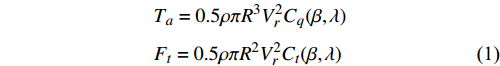
In this section the HAWT benchmark model, detailed in [34], [35] is briefly introduced. The wind kinetic energy is captured by the blades and transferred into the rotor, rotating at ωr. The effective wind speed Vr causes an induced aerodynamic torque Ta and thrust Ft, modelled as
Ta=0.5ρπR3V2rCq(β,λ)Ft=0.5ρπR2V2rCt(β,λ)
(1)
respectively, where ρ is air density and R is blade length. Also, Cq and Ct are torque and thrust coefficients. These coefficients are functions of blade pitch angle, β, and tip speed ratio, λ, defined as λ=Rωr/Vr [2]. Considering the long elastic tower, Ta causes a fore-aft oscillation of the nacelle, i.e., a bending oscillation of the tower. The effective wind speed at the rotor plane is then obtained as Vr=Vw−˙xt, where xt is the nacelle displacement from its equilibrium position, and Vw is the free wind speed, which itself is the wind speed before encountering the blades [10]. It is worth noting that the wind speed measurement by anemometer, installed at the hub, is available on HAWTs. However, due to temporal and spatial distribution of the wind over the blades, tower oscillation, wind shear and tower shadow, there is a significant measurement inaccuracy. So, in this study Vr and consequently Ta are assumed to be unknown.
The captured aerodynamic power by the HAWT is as
Pa=0.5ρπR2V3rCp(β,λ)
(2)
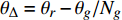
where Cp represents the power coefficient. The drive train (DT) is used to increase the rotor speed ωr and transfer the kinetic energy into the generator shaft, rotating at ωg. The DT is modelled as a two-mass system. The rotor and generator shafts have inertia of Jr and Jg, respectively. The elastic gear meshing is considered, with inclusion of the torsion stiffness Kdt and the torsion damping, Bdt. This elastic gear meshing leads to a torsional angle of twist θΔ, defined as, θΔ=θr−θg/Ng, where, θr and θg are the rotation angle of the rotor and generator shafts, respectively. Also, the viscous friction at the bearings of the rotor and generator shafts are modelled with coefficients Br and Bg, respectively. The DT efficiency is ηdt. So, the DT is modelled as [34]
The rotor kinetic energy is converted into electrical energy in the generator. Additionally, the frequency of the generated power is adjusted using the grid side converter (GSC), located between the generator and the electrical grid [3], [4]. The dynamics of the GSC are modeled as a first-order system with time delay τg to track the requested generator torque load Tg,ref [3], [4]. This does not affect the effectiveness of the methodology, as the benchmark remains a high-fidelity simulator. It is worth noting that the generator's internal electrical faults, manufacturing defects and controller initialization conditions may result in either offsetting the generator torque by fTg(t) or increasing the converter delay by Δτg(t). Though the converter’s controller is typically able to detect and accommodate Δτg(t), the generated power is affected by fTg(t), considerably [7]. So, the converter is modelled as
˙Tg=−agTg+agTg,ref+agfTg
(4)
where ag=1/τg and Tg refers to generator shaft torque. The HAWT internal electronic controller is much faster than the slow mechanical dynamic behavior. Accordingly, the produced electrical power in the generator Pg is approximated as a static relation as
Pg=ηgωgTg
(5)
where ηg is the generator efficiency.
As most of the control schemes are designed based on the feedback of the generator speed measurement [2], sensor faults lead to performance degradation or even instability. Lightning, moisture, salt spray and corrosion, may cause sensor faults. Also, if the encoder is used for shaft speed estimation, degradation of metal pieces on the shaft leads to inaccurate speed measurements. Moreover, malfunctions of the electrical components of the encoders represent another reported source of faults [35]. On the other hand, DT resonance frequency content on the generator speed sensor may deviate the sensor output from accurate readings [36]. The additive time-variable bias is able to represent a variety of sensor faults, i.e., additive constant bias, multiplicative gain changes in the measurements, fixed and no sensor outputs [2]. Therefore, the generator sensor faults are modelled as an additive time-variable bias Δωg(t), corrupting the sensor measurement. For the ease of readability, the HAWT model parameters are summarized in Table I.
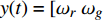
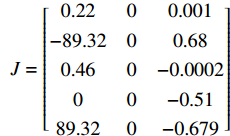
where x(t)=[ωrωgθΔTg]T∈R4 is the system state vector, Tg,ref(t)∈R is the control input, fTg(t)∈R is the actuator fault, Ta(t)∈R represents external disturbance, y(t)=[ωrωgTg]T∈R3 is measurement vector, fs(t)=Δωg(t)∈R is the sensor fault. It should be noted that the measurement error is not included in (6). However, the effect of the measurement error is investigated in the simulation analysis. The known constant dynamics matrices are as follows:
It should be noted that x(t), fa(t), and fs(t) are unknown signals. Although the aerodynamic torque Ta is a given function, this is not computable as it is a function of unknown wind speed. It is worth noting that the wind speed can be measured by anemometer, but it remains a very uncertain signal.
Assumption 1: The actuator fault, sensor fault and aerodynamic torque are bounded, as |fTg|≤ˉfTg, |fs|≤ˉfs, and |Ta|≤ˉTa, where ˉfTg, ˉfs, and ˉTa are unknown positive constants.
Remark 1: Some unknown upper bounds are defined in Assumption 1. To propose a practical solution, in this paper these bounds are assumed to be unknown and will not be used [2].
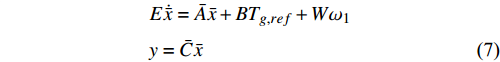
The main objective of this paper is to design an ASMO-based FTC for the HAWT (6). In order to obtain accurate estimates of the faults, the system (6) is augmented into a descriptor form as
E˙ˉx=ˉAˉx+BTg,ref+Wω1y=ˉCˉx
(7)
where ˉx=[xTfs]T∈R5 is the descriptor state, ω1=[fTgTa]T∈R2 is the descriptor disturbance. Also, E=[I404×1]∈R4×5, ˉA=[A04×1]∈R4×5, W=[FaD]∈R4×2, and ˉC=[CFs]∈R3×5 are known constant matrices.
Remark 2: As rank([sI4−AB])=4, ∀s∈C, then the HAWT system (6) is controllable, using the Popov Belevitch Hautus (PBH) lemma [37]. Therefore, having the faults estimated, the generator reference torque Tg,ref and the generator speed sensor ωg are corrected to recover the nominal behavior of the HAWT in the presence of the faults, disturbance and uncertainty. Also, considering Assumption 1, ω1 is bounded as ‖ω1‖≤ˉω1 where ˉω1 is an unknown positive constant.
Now, some technical preliminaries are given, which are used in the ASMO design [38].
Lemma 1: The descriptor system (7) is consistent as EE†(ˉAˉx+BTg,ref+Wω1)=ˉAˉx+BTg,ref+Wω1.
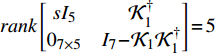
Lemma 2: The descriptor system (7) is impulse observable, since rank[EˉA03×5ˉC04×5E]=size(ˉx)+rank(E). More importantly, as rank[EˉC]=size(ˉx), then system (7) is infinitely observable.
Lemma 3: The triple (E,ˉA,ˉC) is observable, as the system (7) is impulse observable and rank[sE−ˉAˉC]=size(ˉx), ∀s∈C.
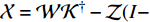
Lemma 4: A necessary and sufficient condition for the existence of a solution for the consistent equation XK=W, with known matrices K and W, is that rank[KW]=rank(K). In this case the general solution is given by X=WK†−Z(I−KK†), where Z is an arbitrary matrix of appropriate dimension.
Remark 3: It is worth noting that Lemma 1 yields that the system (7) is solvable which is sought in Section III. On the other hand, Lemmas 2 and 3 are used in the existence of design matrices (see Lemma 5). Finally, Lemma 4 is useful to find the general solution of a system of algebraic equations (see (12), (13), (15) ,and (16)).
III.
ASMO Design
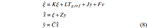
In this section, an ASMO is designed to estimate and reconstruct the descriptor state ˉx and the disturbance ω1. This is fulfilled such that the principle of separation is recovered, i.e., the observer error dynamic response is decoupled from the control input Tg,ref as well as the descriptor state ˉx. Also, the effect of the descriptor disturbance is compensated by design of a discontinuous switching component. Considering the augmented descriptor (7), the ASMO is designed as
˙ξ=Kξ+LTg,ref+Jy+Fνˆˉx=ξ+Zyˆy=ˉCˆˉx
(8)
where ξ∈R5 is the observer state, ˆˉx is the estimate of ˉx, K∈R5×5, L∈R5, J∈R5×3, F∈R5×3, and Z∈R5×3 are design matrices. ν∈R3 is a discontinuous switching component, used to remove the effect of ω1 from the observer performance, designed as
ν=ρνsign(ey)
(9)
where ey is the output estimation error defined as ey=y−ˆy and ρν is a scalar, designed latter. Let us define the transformed estimation error ϵ as ϵ=TEˉx−ξ, where T∈R5×4 is the transformation design matrix. Also, the state estimation error is defined as e=ˉx−ˆˉx.
It follows from (7) and (8) that the estimation error dynamics can be written as:
It is obvious that the state estimation error e is a function of the control input Tg,ref as well as the descriptor state ˉx. In order to recover the principle of separation, i.e., to decouple the dynamics of e from Tg,ref and ˉx, we choose the design matrices of the ASMO (8) to satisfy the following equalities:
TE+ZˉC=I5
JˉC+KTE=TˉA
TB=L.
The matrix equation (11a) can be rearranged as
[TZ]K1=O1
(12)
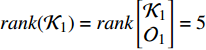
where K1=[EˉC] and O1=I5. Based on Lemma 4, since rank(K1)=rank[K1O1]=5, there exists a solution for (12) with a general form as
[TZ]=O1K†1−R1(I7−K1K†1)
(13)
where R1 represents any real matrix of dimension R5×7. Using the matrix partitioning approach, T and Z are parameterized as
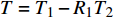
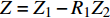
T=T1−R1T2Z=Z1−R1Z2
(14)
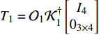
respectively, where the matrices T1, T2, Z1, and Z2 are as T1=O1K†1[I403×4], T2=(I7−K1K†1)[I403×4], Z1=O1K†1[04×3I3], and Z2=(I7−K1K†1)[04×3I3], respectively. From (11a), it is obtained that TE=I5−ZˉC. Substituting this into (11b) yields
[KˉJ]K2=O2
(15)
where ˉJ=J−KZ, O2=TˉA, and K2=[I5ˉC]. Based on Lemma 4, since rank(K2)=rank[K2O2]=5, there exists a solution for (15) with a general form as
[KˉJ]=O2K†2−R2(I8−K2K†2)
(16)
where R2 represents any real matrix of dimension R5×8. Using the matrix partitioning approach, K and ˉJ are parameterized as
K=K1−R2K2ˉJ=ˉJ1−R2ˉJ2
(17)
respectively, where the matrices K1, K2, ˉJ1, and ˉJ2 are as K1=O2K†2[I503×5], K2=(I8−K2K†2)[I503×5], ˉJ1=O2K†2[05×3I3], and ˉJ2=(I8−K2K†2)[05×3I3], respectively.
Obviously, once the matrices R1 and R2 are determined, the observer matrices are obtained by (14) and (17). Therefore, the feasibility of the ASMO (8) is equivalent to the existence of the matrices R1 and R2, which is proved in the following lemma.
Lemma 5: There exist matrices R1 and R2 such that the matrix equalities (11) are satisfied.
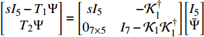
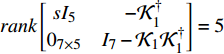
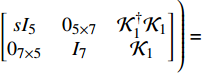
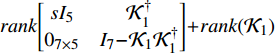
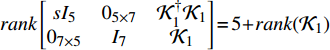
Proof: By using (14) and (17), the matrix K can be written as K=O2K†2[I503×5]−R2K2=(T1−R1T2)ˉAK†2[I503×5]−R2K2. So, it can be shown that K=T1Ψ−R[T2ΨK2], where Ψ=ˉAK†2[I503×5] and R=[R1R2]∈R5×15 is an unknown matrix. Thus, the existence of the matrices R1 and R2 is equivalent to the observability of the pair ([T2ΨK2],T1Ψ). This is equivalent to showing that rank[sI5−T1ΨT2ΨK2]=5, ∀s∈C. This is sufficiently equivalent to the condition rank[sI5−T1ΨT2Ψ]=5. It is easy to show that [sI5−T1ΨT2Ψ]=[sI5−K†107×5I7−K1K†1][I5ˉΨ], where ˉΨ=[I403×4]Ψ. It is clear that rank[I5ˉΨ]=5. Hence, we equivalently prove that rank[sI5−K†107×5I7−K1K†1]=5. Note that
On the other hand, rank[sI505×7K†1K107×5I7K1]=5+rank(K1). Therefore, it can be concluded that, rank[sI5K†107×5I7−K1K†1]=5.■
Now, based on the analysis of ASMO estimation performance, a systematic approach to determine the design matrices K, L, J, F, and Z is given. By satisfying the matrix equalities (11), the estimation error dynamics (10) yields
˙e=Ke+TWω1−Fν.
(18)
We design F=P−1ˉCT and TW=FQ, where P∈R5×5 and Q∈R3×2 are matrices to be designed. With these design matrices the term Qω1 is structurally matched with the control ν, as shown in Theorem 1. Therefore, by a proper design of ν the effect of ω1, i.e., generator fault and aerodynamic torque, can be compensated on the observer estimation performance. Consequently, from (18), it can be pointed out that if the design matrix K is Hurwitz, then the observer accurately estimates ˉx and the error e approaches to zero. The signal ˆˉx contains the estimation of the sensor fault. On the other hand, by exploiting the equivalent output injection approach [29], the generator fault is estimated. The main results are stated in the following theorem.
Theorem 1: Consider the HAWT model (6), represented as the descriptor (7) including the generator torque and sensor simultaneous faults. Under Assumption 1, the ASMO (8) is asymptotically stable and estimates the augmented system state ˉx accurately, if there exists a symmetric positive definite matrix P∈R5×5, a matrix Q∈R3×2 and a positive constant γ, such that
KTP+PK≤−γI5
(19)
PTW=ˉCTQ
(20)
with gain ρν is designed as
ρν=ˆρ+ϵν
(21)
and an adaption law, designed as
˙ˆρ=σ0‖ey‖
(22)
where ˆρ is the estimation of ρ defined as ρ=‖Q‖ˉω1 which is an unknown constant. The matrix F is designed as F=P−1ˉCT. ϵν and σ0 are positive design constants to be selected. Also, ω1 is estimated by
ˆω1=(ˉCP−1ˉCTQ)†(ˉCP−1ˉCTνeq)
(23)
where νeq is the equivalent output injection signal and obtained by passing ν through a designed low pass filter, as νeq=ν/(τcs+1) where τc is a design time constant.
Proof: Choose a positive definite Lyapunov function Vo as
Vo=eTPe+1σ0˜ρ2
(24)
where P∈R5×5 is a symmetric positive definite design matrix and ˜ρ is the estimation error of ρ, defined as ˜ρ=ρ−ˆρ. Taking the time derivative (24) yields
˙Vo=eT(KTP+PK)e+2eTP(TWω1−Fν)−2σ0˜ρ˙ˆρ.
(25)
With the matrix inequality (19) and the adaption law (22), ˙Vo, given in (25), leads to
˙Vo≤−γ‖e‖2+2eTP(TWω1−Fν)−2˜ρ‖ey‖.
(26)
Considering the matrix F designed as F=P−1ˉCT and with the matrix equality (20), (26) can be rewritten as
˙Vo≤−γ‖e‖2+2eTˉCT(Qω1−ν)−2˜ρ‖ey‖.
(27)
From (27) it can be seen that Qω1 is matched with respect to the switching component ν. Therefore, the effect of Qω1 on the observer performance can be totally removed by the design of ν as ν=ρνsign(ey). Also, note that ey=ˉCe. Thus, with gain ρν designed in (21), (27) can be further rewritten as
˙Vo≤−γ‖e‖2−2‖ey‖ϵν≤−γ‖e‖2.
(28)
Thus, taking integration of (28) over [0t] yields to Vo(t)≤Vo(0)−γ∫t0‖e(τ)‖2dτ. Therefore, γ∫t0‖e(τ)‖2dτ≤Vo(0)<∞. Thus, it follows from Barbalat’s lemma [6], that limt→∞e(t)=0 and the ASMO (8) is asymptotically stable. Accordingly, the sliding surface of QTey is reachable and the ASMO (8) estimates the augmented system state ˉx accurately. Therefore, it can be stated that the sensor fault estimation error efs(t)=fs−ˆfs approaches to zero, i.e., limt→∞efs(t)=0. It follows from ey=ˉCe and (18) that:
˙ey=ˉCKe+ˉCTWω1−ˉCFν.
(29)
After the sliding surface is reached, ˙ey=0. Accordingly, (29) leads to
ω1=(ˉCP−1ˉCTQ)†(ˉCP−1ˉCTν−ˉCKe).
(30)
The average behavior of the switching component ν, represented by νeq, can be obtained by passing ν through a low pass filter, as νeq=ν/(τcs+1) where τc is the design time constant. νeq is the necessary effort to maintain the sliding motion or so-called equivalent output injection signal [29]. Hence, ω1 is estimated as
ˆω1=(ˉCP−1ˉCTQ)†(ˉCP−1ˉCTνeq)
(31)
with estimation error eω1(t)=ω1(t)−ˆω1(t)=−(ˉCP−1ˉCTQ)†ˉCKe. As it was proved that the estimation error e approaches to zero, so does eω1. Consequently, ˆω1 is an accurate estimation of ω1. Therefore, it can be shown that the actuator fault estimation error efa(t)=fTg−ˆfTg approaches to zero, i.e., limt→∞efa(t)=0.■
Remark 4: From the stability analysis given in Theorem 1, it is obvious that the dynamic behavior of the convergence of e(t) is governed by γ. By that means, as shown in (28), the larger γ is selected, the faster e(t) approaches to zero. This gives a design freedom such that with appropriate design of γ for the given system, the desirable behavior of the observer is achieved. Indeed, considering (19), γ places the eigenvalues of K away from the imaginary axis in the left half plane and, on the other hand, K determines the estimation error dynamics in (18).
Now, based on the given analysis, the design procedure of ASMO (8) is summarized in Algorithm 1, which is solved offline.
Algorithm 1: ASMO design procedure.
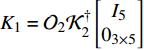
1) Given the matrices E=[I404×1], ˉC=[CFs], and ˉA=[A04×1], compute the matrices K1=[EˉC] , K2=[I5ˉC] , O1=I5,
2) For the given positive constant γ and a small positive constant δ, find a symmetric positive definite design matrix P∈R5×5, design matrices Q∈R3×2, and M∈R5×15, such that they satisfy
X1+X1T<−γI5
(32)
0<[δI5X2X2TδI2]
(33)
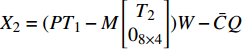
where X1=PT1Ψ−M[T2ΨK2], X2=(PT1−M[T208×4])W−ˉCQ.
3) Compute R1 and R2 as R1=P−1M[I708×7], R2=P−1M[07×8I8].
4) Compute the matrices T=T1−R1T2, O2=TˉA, K1=O2K†2[I503×5], and ˉJ1=O2K†2[05×3I3].
5) Compute the ASMO matrices Z=Z1−R1Z2, K=K1−R2K2, and ˉJ=ˉJ1−R2ˉJ2. Then, compute J=ˉJ+KZ, F=P−1ˉCT, and L=TB.
Note that in Algorithm 1, the matrix equality (20) is replaced with the equivalent matrix inequality (33) [39]. On the other hand, to have design freedom, the small positive constant δ is given without loss of accuracy. Nevertheless, it can be replaced with a minimization with respect to δ. Also, the design matrix M is defined as M=PR for ease of implementation, where R=[R1R2]∈R5×15 is the design matrix to be used in (14) and (17).
IV.
Nominal Behavior Recovery
In this section, the FTC scheme is designed, using the signal correction procedure, to recover the nominal behavior of the HAWT, despite the occurrence of the faults. As discussed earlier, it is aimed to keep the HAWT nominal controller in use, to ensure industrial acceptability. In this manner, the nominal controller is briefly recalled. For the wind speed lower that the nominal value, the operational objective is to maximize the captured power. On the other hand, for high wind speed values, it is aimed to maintain the generated power at its nominal value. The former objective is achieved by regulating the reference generator torque, i.e., Tg,ref, while the latter one is achieved by regulating the reference pitch angle of the blades, i.e., βref. Then, the nominal controller in low wind speed situation is as
Tg,ref(ωg)=Kcω2g(t)βref=0
(34)
and in high wind speed situation is as
Tg,ref=Tg,Nβref(ωg)=Kpeωg(t)+Ki∫t0eωg(τ)dτ
(35)
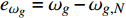
where Kc=0.5ρπηdtR5CP,max/N3gλ3opt is a constant gain, obtained based on the HAWT parameters, such that CP,max is the maximum power coefficient achieved at the optimal tip speed ratio λopt. Kp and Ki are PI controller gains, and eωg=ωg−ωg,N is the tracking error [40]. Also, ωg,N and Tg,N are the rated generator speed and torque values, respectively [40], [41]. It is worth noting that the stability of the nominal controller is already guaranteed. To avoid repetition, specific details can be found in [34], [35].
It is obvious that the presence of the generator speed sensor fault perturbs the performance of the nominal controller. Additionally, the generator torque fault causes deviation from the maximum power generation. It is worth noting that the generator torque fault degrades the nominal power generation and quality of the generated power for high wind speed situations. Accordingly, it is desirable to remove the generator simultaneous sensor and actuator faults, and then, to recover the normal behavior. Also, we aim to have nominal behavior recovery achieved using the nominal controller (34) and (35). In this sense, the generator speed measurement is modified before being fed back into the nominal controller as
ωg,m=ωg−ˆfs.
(36)
Consequently, the FTC scheme is designed as
Tg,FTC=Tg,ref(ωg,m)−ˆfTgβFTC=βref(ωg,m).
(37)
It is evident from (37) that the nominal controller structure is kept in use, and it is only reconfigured to recover the nominal behavior. The performance of the ASMO-based FTC approach (37) is addressed in Theorem 2.
Theorem 2: Consider the HAWT dynamics (6), equipped with ASMO (8) and FTC scheme (37) under Assumption 1. When the generator sensor fault fs and actuator fault fTg occur, the closed-loop system asymptotically recovers the nominal behavior of the HAWT after the sliding surface of QTey is reached.
Proof: Substituting (37) into (6) yields
˙x(t)=Ax(t)+BTg,ref(t)+DTa(t)+χ(efs,efa)
(38)
where χ(efs,efa)=BKce2fs+2BKcωgefs+Befa. Since it was proven in Theorem 1 that efs and efa asymptotically approach to zero, then limt→∞χ(∙)=0. Thus, the closed-loop system (38) becomes
˙x(t)=Ax(t)+BTg,ref(t)+DTa(t)
(39)
which is exactly the nominal behavior, i.e., the fault-free condition of (6). As the stability of the nominal controller is guaranteed, by having the nominal behavior recovered, the stability of the closed-loop system is achieved.■
Remark 5: Within this structure, the nominal controllers (34) and (35) can be replaced by any of the other modern designs available in the literature. This represents a significant feature of the proposed scheme, since it is based on the decoupling approach. This also gives a design freedom, i.e., a variety of available industrial controllers can be kept in use.
V.
Simulation
In this section, the performance of the proposed approach is evaluated by implementing it to the 4.8 MW HAWT benchmark, whose technical specifications are illustrated in [7], [34]. It should be noted that the low wind speed case is considered, as the generator sensor and actuator faults have considerable effects. Nevertheless, the proposed solution is applicable for the whole operational region of the HAWT, i.e., low and high wind speed. The generator sensor and actuator faults are defined as
respectively. It is worth noting that in [5], [15], [34], [35] the faults are modelled as a constant bias. However, in this paper to account for a wide variety of time varying faults, we consider the above-mentioned fault signals. Also, to investigate the solution practically, the sensor measurement errors are modelled as Gaussian noise processes, with zero mean and standard deviation, σωr=0.2, σωg=0.05, and σTg=5 for rotor speed, generator speed, and generator torque measured signals, respectively [34], [35]. The ASMO design parameters are as follows:
Also, σ0=1000, ϵν=1, and τc=0.01. The wind speed profile is shown in Fig. 1. Moreover, the generated power with and without the proposed solution are illustrated in Fig. 2. It is evident that the effect of the sensor fault is considerable. This is due to the fact that in the nominal control (34) the sensor measurement is squared and multiplied by Kc. In order to accurately compare the results, the approach presented by Shi and Patton in [15] is used as well. The achieved result by applying this approach is shown in Fig. 2 (black dashed line). It is worth noting that even though in [15] the observer is designed, the robustness is achieved by the H∞ optimization approach. More importantly, separate faults were considered. This issue is obvious in Fig. 2. Indeed, the approach in [15] satisfactorily suppresses the effects of separate faults. However, when simultaneous faults are applied, this approach performance degrades. In contrast, it is evident that our solution is able to actively compensate for the effects of faults, occurring either separately or simultaneous.
Figure
1.
The wind speed profile of the benchmark model.
To illustrate the effect of generator actuator faults, in Figs. 3 and 4, the generated power in the time periods 40(s)<t<50(s) and 90(s)<t<100(s) are shown, respectively. It should be pointed out that in the mentioned time periods, considering the definition of fs and fa, the generator actuator faults are only active.
The estimated sensor and actuator faults are compared to the actual ones in Figs. 5 and 6, respectively. It can be seen that the nominal operation of the HAWT benchmark is recovered using the proposed approach. Moreover, the sensor and actuator faults are accurately estimated. To precisely investigate the effectiveness of the proposed FTC, Tg,ref is illustrated in Fig. 7. It can be noted that in the faulty periods the Tg,ref is corrected corresponding to the estimated faults to remove their effects.
Figure
5.
Actual and estimated sensor fault of fs.
The different cases of Monte-Carlo simulation are summarized in Table II. Three sets of measurement noise standard deviations are considered, which are described as Set1={σωr=1(2.5%),σωg=0.5(4%),σTg=10(1%)}, Set2={σωr=4(10%),σωg=1(8%),σTg=20(2%)}, and Set3={σωr=8(20%),σωg=2(16%),σTg=40(4%)}. The Monte-Carlo simulation is performed under the occurrence of the generator sensor and actuator faults. For each case, 60 runs are considered. To compare the results numerically, the normalized power metric (PM) is computed as
where Pg,ff is the generated power in the fault-free condition. Then, the maximum, minimum, mean and standard deviation of the PM is computed. For the sake of brevity, the worst (W), the average (A), and the best (B) values are summarized in Table II. All results presented in Table II show small values of the PM, i.e., limited variation of the generated power in the faulty case with respect to the corresponding one in the fault-free situation. Moreover, Table II highlights the robustness of the proposed approach with respect to measurement errors, wind speed variations as well as faults. It is worth noting that the variations of PM are smaller than the variations of the noise within the considered data sets (Set1, Set2, and Set3).
VI.
Conclusions and Future Research Directions
In this paper, an adaptive sliding mode observer was designed, enabling the estimation of generator actuator and sensor simultaneous faults. As the principle of separation was recovered by the proposed scheme, the nominal controller was kept in use for the fault tolerance purpose, recovering the nominal behavior of the wind turbine in the presence of faults. The accurate measurement or estimation of the unknown wind speed and consequent unknown aerodynamic torque was not required. This led to a simple and less computationally-expensive scheme which can be used in industry. The effectiveness of the proposed scheme was numerically evaluated using a 4.8 MW wind turbine benchmark model. The reliability and robustness characteristics of the proposed approach against measurement errors were further assessed using the Monte-Carlo analysis. The results showed that the nominal operation was recovered using the proposed approach, in the presence of simultaneous faults and the unknown wind speed variations. Sensor and actuator faults were also accurately estimated using the proposed observer. The contributions of this paper can motivate the following future research directions. For instance, a necessary step to the industrial deployment of the proposed scheme is its experimental validation, with cost analysis and assessment of the economic benefits. This includes the analysis of other faults, the computation of the downtime/availability, and operation costs. This, cumulatively, leads to estimation of the average wind turbine lifespan. On the other hand, the proposed approach can further be extended to the high wind speed region, where the pitch actuator is active. Finally, further Monte-Carlo analysis can be performed to assess other performance metrics, such as false alarm rates, missed fault rates and detection delays.
B. Yang, T. Yu, H. Shu, J. Dong, and L. Jiang, “Robust slidingmode control of wind energy conversion systems for optimal power extraction via nonlinear perturbation observers,” Appl. Energy, vol. 210, pp. 711–723, 2018. doi: 10.1016/j.apenergy.2017.08.027
[2]
H. Habibi, I. Howard, and S. Simani, “Reliability improvement of wind turbine power generation using model-based fault detection and fault tolerant control: A review,” Renew. Energy, vol. 135, pp. 877–896, 2019. doi: 10.1016/j.renene.2018.12.066
[3]
M. J. Morshed and A. Fekih, “A sliding mode approach to enhance the power quality of wind turbines under unbalanced voltage conditions,” IEEE/CAA J. Autom. Sinica, vol. 6, no. 2, pp. 566–574, 2019. doi: 10.1109/JAS.2019.1911414
[4]
M. J. Morshed, “A nonlinear coordinated approach to enhance the transient stability of wind energy-based power systems,” IEEE/CAA J. Autom. Sinica, vol. 7, no. 4, pp. 1087–1097, 2020. doi: 10.1109/JAS.2020.1003255
[5]
H. Badihi, Y. Zhang, and H. Hong, “Fault-tolerant cooperative control in an offshore wind farm using model-free and model-based fault detection and diagnosis approaches,” Appl. Energy, vol. 201, pp. 284–307, 2017. doi: 10.1016/j.apenergy.2016.12.096
[6]
J. Lan, R. J. Patton, and X. Zhu, “Fault-tolerant wind turbine pitch control using adaptive sliding mode estimation,” Renew. Energy, vol. 116, pp. 219–231, 2018. doi: 10.1016/j.renene.2016.12.005
[7]
C. Sloth, T. Esbensen, and J. Stoustrup, “Robust and fault-tolerant linear parameter-varying control of wind turbines,” Mechatronics, vol. 21, no. 4, pp. 645–659, 2011. doi: 10.1016/j.mechatronics.2011.02.001
[8]
H. Habibi, H. R. Nohooji, and I. Howard, “A neuro-adaptive maximum power tracking control of variable speed wind turbines with actuator faults,” in Proc. Australian and New Zealand Control Conf., Gold Coast, Australia, 2017, pp. 63–68.
[9]
H. Habibi, H. R. Nohooji, and I. Howard, “Constrained control of wind turbines for power regulation in full load operation,” in Proc. 11th Asian Control Conf., Australia, 2017, pp. 2813–2818.
[10]
M. S. Mahmoud and M. O. Oyedeji, “Adaptive and predictive control strategies for wind turbine systems: A survey,” IEEE/CAA J. Autom. Sinica, vol. 6, no. 2, pp. 364–378, 2019. doi: 10.1109/JAS.2019.1911375
[11]
U. Giger, P. Kühne, and H. Schulte, “Fault tolerant and optimal control of wind turbines with distributed high-speed generators,” Energies, vol. 10, no. 2, pp. 1–13, 2017.
[12]
F. Jaramillo-Lopez, G. Kenne, and F. Lamnabhi-Lagarrigue, “A novel online training neural network-based algorithm for wind speed estimation and adaptive control of PMSG wind turbine system for maximum power extraction,” Renew. Energy, vol. 86, pp. 38–48, 2016. doi: 10.1016/j.renene.2015.07.071
[13]
Y.-M. Kim, “Robust data driven H-infinity control for wind turbine,” J. Franklin Inst., vol. 353, no. 13, pp. 3104–3117, 2016. doi: 10.1016/j.jfranklin.2016.06.009
[14]
M. A. Soliman, H. M. Hasanien, H. Z. Azazi, E. E. El-Kholy, and S. A. Mahmoud, “An adaptive fuzzy logic control strategy for performance enhancement of a grid-connected PMSG-based wind turbine,” IEEE Trans. Industr. Inform., vol. 15, no. 6, pp. 3163–3173, 2018.
[15]
F. Shi and R. Patton, “An active fault tolerant control approach to an offshore wind turbine model,” Renew. Energy, vol. 75, pp. 788–798, 2015. doi: 10.1016/j.renene.2014.10.061
[16]
X. Liu, Z. Gao, and M. Z. Chen, “Takagi–Sugeno fuzzy model based fault estimation and signal compensation with application to wind turbines,” IEEE Trans. Ind. Electron., vol. 64, no. 7, pp. 5678–5689, 2017. doi: 10.1109/TIE.2017.2677327
[17]
F. D. Bianchi, H. De Battista, and R. J. Mantz, Wind Turbine Control Systems: Principles, Modelling and Gain Scheduling Design, London, UK: Springer Science and Business Media, 2006.
[18]
D. Song, J. Yang, Z. Cai, M. Dong, M. Su, and Y. Wang, “Wind estimation with a non-standard extended Kalman filter and its application on maximum power extraction for variable speed wind turbines,” Appl. Energy, vol. 190, pp. 670–685, 2017. doi: 10.1016/j.apenergy.2016.12.132
[19]
V. Nikolić, S. Motamedi, S. Shamshirband, D. Petković, S. Ch, and M. Arif, “Extreme learning machine approach for sensorless wind speed estimation,” Mechatronics, vol. 34, pp. 78–83, 2016. doi: 10.1016/j.mechatronics.2015.04.007
[20]
O. Barambones, “Robust wind speed estimation and control of variable speed wind turbines,” Asian J. Control, vol. 21, no. 2, pp. 856–867, 2019. doi: 10.1002/asjc.1779
[21]
Z. Gao, X. Liu, and M. Chen, “Unknown input observer-based robust fault estimation for systems corrupted by partially decoupled disturbances,” IEEE Trans. Ind. Electron., vol. 63, no. 4, pp. 2537–2547, 2015.
[22]
B. Marx, D. Ichalal, J. Ragot , D. Maquin, and S. Mammar, “Unknown input observer for LPV systems,” Automatica, vol. 100, pp. 67–74, 2019. doi: 10.1016/j.automatica.2018.10.054
[23]
Z. Li and J. Zhao, “Fuzzy adaptive robust control for stochastic switched nonlinear systems with full-state dependent nonlinearities,” IEEE Trans. Fuzzy Sys., vol. 28, no. 9, pp. 2035–2047, 2020. doi: 10.1109/TFUZZ.2019.2930034
[24]
Y. Zhang , T. Zeng, and G. Li, “Robust excitation force estimation and prediction for wave energy converter m4 based on adaptive slidingmode observer,” IEEE Trans. Industr. Inform., vol. 16, no. 2, pp. 1163–1171, 2020. doi: 10.1109/TII.2019.2941886
[25]
L. Chen, X. Huang, and M. Liu, “Fault-tolerant control against simultaneous partial actuator degradation and additive sensor fault,” in Proc. American Control Conf., 2017, pp. 4105–4110.
[26]
Y. Wang, Y. Xia, H. Li, and P. Zhou, “A new integral sliding mode design method for nonlinear stochastic systems,” Automatica, vol. 90, pp. 304–309, 2018. doi: 10.1016/j.automatica.2017.11.029
[27]
J. Lan and R. J. Patton, “A new strategy for integration of fault estimation within fault-tolerant control,” Automatica, vol. 69, pp. 48–59, 2016. doi: 10.1016/j.automatica.2016.02.014
[28]
A. F. De Loza, J. Cieslak, D. Henry, A. Zolghadri, and L. M. Fridman, “Output tracking of systems subjected to perturbations and a class of actuator faults based on HOSM observation and identification,” Automatica, vol. 59, pp. 200–205, 2015. doi: 10.1016/j.automatica.2015.06.020
[29]
S. Yin, H. Gao, J. Qiu, and O. Kaynak, “Descriptor reduced-order sliding mode observers design for switched systems with sensor and actuator faults,” Automatica, vol. 76, pp. 282–292, 2017. doi: 10.1016/j.automatica.2016.10.025
[30]
Z. Huang, R. J. Patton, and J. Lan, “Sliding mode state and fault estimation for decentralized systems,” in Variable-Structure Approaches, Springer, 2016, pp. 243–281.
[31]
W. H. Chen, J. Yang, L. Guo, and S. Li, “Disturbance-observer-based control and related methods an overview,” IEEE Trans. Indust. Elect., vol. 63, no. 2, pp. 1083–1095, 2016. doi: 10.1109/TIE.2015.2478397
[32]
P. Kühne, F. Pöschke, and H. Schulte, “Fault estimation and fault-tolerant control of the FAST NREL 5 MW reference wind turbine using a proportional multi-integral observer,” Int. J. Adapt. Contr. Signal Process., vol. 32, no. 4, pp. 568–585, 2018. doi: 10.1002/acs.2800
[33]
S. Zhang and Z. Q. Lang, “SCADA-data-based wind turbine fault detection: A dynamic model sensor method,” Control. Eng. Pract., vol. 102, Article No. 104546, 2020. doi: 10.1016/j.conengprac.2020.104546
[34]
P. F. Odgaard and J. Stoustrup, “A benchmark evaluation of fault tolerant wind turbine control concepts,” IEEE Trans. Cont. Syst. Tech., vol. 23, no. 3, pp. 1221–1228, 2015. doi: 10.1109/TCST.2014.2361291
[35]
P. F. Odgaard, J. Stoustrup, and M. Kinnaert, “Fault-tolerant control of wind turbines: A benchmark model,” IEEE Trans. Contr. Syst. Tech., vol. 21, no. 4, pp. 1168–1182, 2013. doi: 10.1109/TCST.2013.2259235
[36]
V. Pashazadeh, F. R. Salmasi, and B. N. Araabi, “Data driven sensor and actuator fault detection and isolation in wind turbine using classifier fusion,” Renew. Energy, vol. 116, pp. 99–106, 2018. doi: 10.1016/j.renene.2017.03.051
[37]
V. Joukov, J. Ćesić, K. Westermann, I. Marković, I. Petrović, and D. Kulić, “Estimation and observability analysis of human motion on Lie groups,” IEEE Trans. Cybernetics, vol. 50, no. 3, pp. 1321–1332, 2019.
[38]
M. Darouach and T. Fernando, “On the existence and design of functional observers,” IEEE Trans. Auto. Contr., vol. 65, no. 6, pp. 2751–2759, 2019.
[39]
J. Lan and R. J. Patton, “A decoupling approach to integrated faulttolerant control for linear systems with unmatched non-differentiable faults,” Automatica, vol. 89, pp. 290–299, 2018. doi: 10.1016/j.automatica.2017.12.011
[40]
H. Habibi, A. Y. Koma, and I. Howard, “Power improvement of nonlinear wind turbines during partial load operation using fuzzy inference control,” Control Eng. Appl. Inf., vol. 19, no. 2, pp. 31–42, 2017.
[41]
H. Habibi, I. Howard, and R. Habibi, “Bayesian fault probability estimation: Application in wind turbine drivetrain sensor fault detection,” Asian J. Control, vol. 22, no. 2, pp. 624–647, 2020. doi: 10.1002/asjc.1973
A simple design enabling the detection of simultaneous sensor and actuator faults,
Recovering the principle of separation and enabling the use of the nominal controller,
Easy to implement and computationally-inexpensive wind turbine control design.
Export File
Citation
Hamed Habibi, Ian Howard, Silvio Simani, and Afef Fekih, "Decoupling Adaptive Sliding Mode Observer Design for Wind Turbines Subject to Simultaneous Faults in Sensors and Actuators," IEEE/CAA J. Autom. Sinica, vol. 8, no. 4, pp. 837-847, Apr. 2021. doi: 10.1109/JAS.2021.1003931
Hamed Habibi, Ian Howard, Silvio Simani, and Afef Fekih, "Decoupling Adaptive Sliding Mode Observer Design for Wind Turbines Subject to Simultaneous Faults in Sensors and Actuators," IEEE/CAA J. Autom. Sinica, vol. 8, no. 4, pp. 837-847, Apr. 2021. doi: 10.1109/JAS.2021.1003931


 DownLoad:


 DownLoad:


 DownLoad:


