


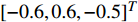
Figure
1.
Network architecture of USNs.
 Volume 7
Issue 6
Volume 7
Issue 6
IEEE/CAA Journal of Automatica Sinica
| Citation: | Haiyan Zhao, Jing Yan, Xiaoyuan Luo and Xinping Guan, "Privacy Preserving Solution for the Asynchronous Localization of Underwater Sensor Networks," IEEE/CAA J. Autom. Sinica, vol. 7, no. 6, pp. 1511-1527, Nov. 2020. doi: 10.1109/JAS.2020.1003312

|
INTERNET of underwater things (IoUTs) is defined as a world-wide network that incorporates underwater physical process, ubiquitous computation, efficient communication and reliable control [1]. In IoUTs, one of the most promising technologies is to utilize underwater sensor networks (USNs) to monitor the sea area. The USNs can support applications in various areas such as marine resource protection, gas and oil spill monitoring, data collection, disaster warning and mine reconnaissance (see [2]–[6] and references therein). For the applications of USNs, the precise localization of sensor nodes has become one of the primary prerequisites. This critical importance arises from its fundamental role in the sensing, communication and control of vast unexplored ocean volume, because these commands are valid only when the location information of sensor nodes is accurate.
In general, the localization schemes developed for sensor networks that can achieve high-accuracy localization are based on time. The time-based schemes employ various mechanisms such as time of arrival (TOA), time of flight (TOF), or time difference of arrival (TDOA) to measure distances. Since the distance measurement is derived from the time (or time difference), the time-based schemes rely heavily on the clock synchronization assumption of sensor nodes. For terrestrial sensor networks, the clock synchronization assumption can be easily founded through the assistance of global positioning system (GPS). However, the unique characteristics of USNs make underwater localization more [7]. For instance, radio waves are strongly absorbed in water, and GPS technology is not available for USNs. Moreover, the propagation delay of acoustic speed (
In order to achieve effective localization for IoUTs, some asynchronous localization algorithms have been developed, e.g., [12]–[15]. These algorithms mainly involve the following process. 1) Anchor discovery: several non-collinear anchor nodes are deployed in the network to provide localization reference for sensor nodes; 2) Distance measurement: the distance measurements are derived by multiplying the time (or time difference) with the transmission speed; 3) Location estimation: with the positions of anchor nodes and the measured distances, optimal or suboptimal estimators are designed to calculate the locations of sensor nodes. In such a process, the privacy preservation is not taken into consideration, since the positions of anchor nodes are directly revealed to the networks. However, the USNs are usually deployed in harsh or even insecure environment, and security threats cannot be avoided. Ignoring the effect of privacy preservation can lead to privacy leakage or even failure of the localization [16]. For example, malicious nodes can easily attack the anchor nodes and destroy the whole localization system if they harvest the locations of anchor nodes. Inspired by this, many privacy-preserving localization schemes have been proposed. For instance, the encryption technique was adopted in [17] and [18], through which privacy-preserving schemes were designed for indoor localization. In [19] and [20], the privacy preserving summation (PPS) strategy was employed to hide private location information of anchor nodes. Nevertheless, the localization schemes in [17]–[20] relied on the assumption of synchronous clock, i.e., the transmitter-receiver synchronization was assumed to be ensured. Meanwhile, the mobility characteristic of nodes was not considered in [17]–[20], i.e., the nodes were assumed to be static. As mentioned above, the clocks in USNs are always asynchronous, wherein the nodes often have passive motions. Ignoring the above characteristics can increase ranging errors and reduce localization accuracy. Per knowledge of the authors, how to design a localization algorithm that jointly considers the asynchronous clock, mobility and privacy preservation is not well studied.
This paper develops a privacy preserving solution for the asynchronous localization of USNs. We first present a hybrid network architecture, which includes four types of nodes, i.e., surface buoys, anchors, active sensors and ordinary sensors. In order to eliminate the effects of asynchronous clock and mobility, an asynchronous localization protocol is developed, through which PPS and privacy-preserving diagonal product (PPDP) based localization algorithms are designed to hide privacy information. Main contributions lie in two aspects:
1) Asynchronous Localization Protocol With the Consideration of Asynchronous Clock and Mobility: An asynchronous localization protocol is provided to eliminate the effect of asynchronous clock and mobility, through which the relationship between propagation delay and location is constructed. Different from the existing works [17]–[20], the clocks between anchors and sensors are not required to be synchronized. Meanwhile, the proposed localization protocol in this paper can compensate both the influences of clock skew and offset as compared with the works [12], [13], [21].
2) Asynchronous Localization Algorithm With the Consideration of Privacy Preservation: Without adopting any homomorphic encryption technique, PPS and PPDP based asynchronous localization algorithms are designed for USNs to hide the private location information. Compared to the existing works [14], [15], the position information of anchor nodes in this paper does not require to be revealed. Per knowledge of the authors, this is the first work that employs privacy preservation strategy into the asynchronous localization of USNs.
Recently, the localization of terrestrial sensor networks has been extensively investigated. For instance, a divide-and-conquer strategy that enabled sparse localization of sensor nodes was developed in [22]. In [23], a viable kernel-based algorithm was presented to solve the localization problem. Also of relevance, some other localization algorithms were proposed for terrestrial sensor networks (see [24] and the references therein). However, these algorithms cannot be directly applied to USNs due to the unique characteristics of underwater environment. In the following, we review literatures on the topic of asynchronous localization of USNs.
In [21], a silent localization scheme was developed, where the underwater sensor nodes did not actively transmit any message. Based on this, an on-demand asynchronous localization (ODAL) scheme was provided in [12]. It can be seen that the mobility characteristic of USNs in [12], [21] was not considered. To handle this issue, Tsai et al. [25] developed a hybrid mobile localization algorithm for USNs. In [26], a prediction-based localization algorithm called scalable localization with mobility prediction (SLMP) was designed to predict the locations of sensor nodes. More recently, a mobility prediction based asynchronous localization algorithm was given in [13]. Nevertheless, the clock model in [12], [13], [21], [25], [26] ignored the clock skew, and this assumption can increase the synchronization error when the localization window was not small. With this consideration, some joint localization and synchronization algorithms have been proposed. For instance, a multi-phase solution to localization and synchronization was presented in [14], where the clock skew and offset were both considered. Different from [14], a unified framework was presented in [27], where the localization and synchronization tasks can be achieved simultaneously. In [28], an autonomous underwater vehicle (AUV) was employed as the anchor node, through which an AUV-aided asynchronous localization strategy was presented. Reference [29] studied a joint localization and tracking issue for AUV. In order to reduce the linearization errors, a follow-up work [30] was given to present an unscented transform-based asynchronous localization algorithm. Also of relevance, some underwater asynchronous localization algorithms were proposed in [31]–[33]. However, the major focus in the above studies is the design of communication protocol to localize sensor nodes, where the privacy preservation issue is not considered. It is worth mentioning that, the privacy preservation is critical for the success of localization process. With consideration of the mobility, how to incorporate the privacy preservation into the asynchronous localization of USNs is largely unexplored.
To avoid information leakage, some privacy-preserving localization [17], [18] adopted homomorphic encryption technique to hide the position information of indoor sensor nodes. Other encryption technique-based privacy preservations were developed in [16], [34]–[36]. Although the encryption technique can provide strong privacy preservation performance, its communication and computational overheads are high. Thereby, the encryption technique is not suitable for underwater localization [16], due to the limited bandwidth and energy of USNs. Inspired by this, some researchers attempt to use the signal processing solutions to preserve privacy data, whose main idea is to add noises to the privacy data. For instance, the authors in [19], [20] adopted PPS into TDOA-based localization, through which two privacy-preserving least squares estimators were designed. In [37], a privacy preserving mechanism was presented for the position estimation, and a differential privacy based privacy-preserving indoor localization scheme was designed in [38]. Nevertheless, these studies rely on the synchronous assumption, and they cannot be directly applied to the asynchronous localization. This paper gives a privacy-preserving localization solution for USNs, and more importantly, we consider more complex but realistic underwater environment, i.e., asynchronous clock and mobility characteristics.
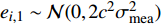
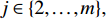
In order to realize privacy-preserving asynchronous localization for USNs, we provide a network architecture that includes four different types of nodes, as depicted in Fig. 1.
1) Surface Buoys: Surface buoys are installed with GPS to acquire their accurate time references and positions through electromagnetic communication. The role of surface buoys is to provide self-localization and clock synchronization services for anchor nodes.
2) Anchor Nodes: Anchor nodes are powerful fixed nodes, and they make direct communication with surface buoys. Similar to the assumption in [26], [39], it is assumed that the time clocks of anchor nodes are synchronized and the locations are pre-known by using some existing technologies, e.g., the localization approach in [40].
3) Active Sensor Node: Active sensor nodes initiate the whole localization process by broadcasting timestamps to the networks. Due to the effect of water current, active sensor nodes can move passively, whose velocities can be accurately measured by Doppler velocity log (DVL) or fiber optic gyroscope (FOG). Particularly, the locations of active sensor nodes are required to be estimated and protected. It is emphasized that the clocks of active sensor nodes are not well synchronized with the real time.
4) Ordinary Sensor Nodes: Ordinary sensor nodes are low-complexity nodes, and they cannot initiatively start the whole localization process, i.e., they just passively listen to the networks and then send state noises to anchor nodes. The locations of ordinary sensor nodes are required to be estimated and protected. Similar to active sensor nodes, ordinary sensor nodes can move passively, whose velocities can be accurately measured. Besides, the clocks of ordinary sensor nodes are asynchronous.
With the above network architecture, the localization process is divided into two subprocesses: a) active sensor localization; b) ordinary sensor localization. Without loss of generality, one active sensor node and one ordinary sensor node are considered here, while the method for single node can be easily extended to the other nodes. Besides, each node can hear message only from its neighboring nodes, i.e., each node cannot hear everybody else due to its limited sensing range. Thus, it is assumed that
At the beginning, active sensor node sends out an initiator message to its neighboring nodes. Upon receiving the initiator message, anchor nodes record and reply the initiator message. Meanwhile, ordinary sensor node passively listens to the messages from active sensor node and anchor nodes. Since the exchange process can be quickly completed, it assumed that the positions of active and ordinary sensor nodes are fixed during the timestamp exchange process. The timestamp transmission process can be illustrated by Fig. 2, and some important notations are listed in Table I. Accordingly, the asynchronous localization protocol is detailed as follows.
| Notation | Description | |
| Ta,a | Time when active sensor sends initiator message | |
| ta,i | Time when anchor i receives initiator message | |
| ti,i | Time when anchor i sends message | |
| tj,i | Time when anchor i receives message from anchor j | |
| Ti,a | Time when active sensor receives message from anchor i | |
| Ta,p | Time when ordinary sensor receives message from active sensor | |
| Ti,p | Time when ordinary sensor receives message from anchor i | |
| ϖi,1 | Time measurement noise between anchor i and anchor 1 | |
| ϖi,p | Time measurement noise between anchor i and ordinary sensor |
 DownLoad:
CSV
DownLoad:
CSV

1) At time
2) At time
3) At time
| Ta,a,{ta,i,ti,i,Ti,a,tr,i}mi=1,{tj,i}m,i−1i=2,j=1,tr. | (1) |
4) Ordinary sensor node passively listens to the networks, and it sends out state noises to anchor nodes as required. Accordingly, ordinary sensor node has the following timestamp measurements from anchor nodes
| Ta,a,Ta,p,{ta,i,ti,i,Ti,p,tr,i}mi=1,{tj,i}m,i−1i=2,j=1,tr. | (2) |
5) With the collected timestamps in (1) and (2), two asynchronous localization algorithms are given to estimate the positions of active and ordinary sensor nodes at timestamps
Different from the simplified model in [12], [13], [21], a clock model including time skew and offset is considered
| Ta=αat+βa,Tp=αpt+βp | (3) |
where
Remark 1: It is noted that, the asynchronous localization protocol in this paper is similar to the ones in [12], [13], [30]. Nevertheless, the asynchronous localization protocol in this paper is essentially different from the ones in [12], [13], [30]. Two reasons are associated with this judgement: 1) The clock model in [12], [13] ignores the clock skew (i.e.,
Due to the mobility characteristic, the above localization protocol should be periodically enforced to update the position information. However, this implementation can result in a waste of communication costs. In order to handle this issue, we develop a mobility compensation strategy, whose aim is to balance the tradeoff between communication cost and localization accuracy. Then, the time axis is divided into multiple measurement windows with length set to
| pT∗a,a={pa,if(T∗a,a−Ta,a)<δαapa+δαana∑ma=0va(→Ta,a),otherwise | (4) |
where

Similar to the active sensor node, the position vectors of ordinary sensor node at timestamps
| pT∗a,p={pp,if(T∗a,p−Ta,p)<δαppp+δαpnp∑mp=0vp(→Ta,p),otherwise | (5) |
where
With the above localization protocol, the following two problems require to be solved for the localization algorithms.
Problem 1 (Privacy-Preserving Asynchronous Localization for Active Sensor Node): In USNs, the clocks are asynchronous and the position information is required to be protected. Inspired by this, we attempt to design a privacy-preserving asynchronous localization algorithm for active sensor node, where active sensor node initiates the localization process by broadcasting message to the networks. This problem is reduced to the estimation of
Problem 2 (Privacy-Preserving Asynchronous Localization for Ordinary Sensor Node): Different from the active sensor node, the ordinary sensor node cannot initiatively broadcast timestamps to the networks. Thereby, the localization algorithm designed for active sensor node is not suitable for ordinary sensor node. Inspired by this, we aim to design a privacy-preserving asynchronous localization algorithm for ordinary sensor node. This problem can be reduced to the estimation of
We first present a PPS-based asynchronous localization algorithm for active sensor node. Note that the PPS-based localization is not suitable for ordinary sensor node. Then, a PPS and PPDP based asynchronous localization algorithm is designed for ordinary sensor node. Finally, we present the consequence when there exist dishonest nodes.
In order to remove the effect of asynchronous clock, we define the following time difference, i.e.,
| ΔTi,1=ta,i−ta,1,i∈{2,…,m}. | (6) |
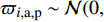
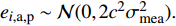
Without loss of generality, we assume that all nodes including anchor nodes, active and ordinary sensor nodes have the same measurement quality. Particularly, the measurement noise of each local measurement is a random variable with zero mean and variance
| ΔTi,1=(ta,a+trαa+τa,i+ϖa,i)−(ta,a+trαa+τa,1+ϖa,1)=τa,i−τa,1+ϖi,1 | (7) |
where
With (7), we have the following distance difference
| Υi,1=da,i−da,1+ei,1,i∈{2,…,m} | (8) |
where
It is denfined that
| minxam∑i=2((Υi,1+da,1)2−d2a,i)2. | (9) |
Denote the position vector of anchor node
| minxa‖2Axa−B‖2 | (10) |
where
By employing the traditional LS estimator, the direct estimation of
| ˆxa,direct=12(ATA)−1ATB. | (11) |
However, the direct calculation of
| ˆxa,indirect=12˜A−1˜B. | (12) |
With regard to (12), the main process of PPS-based asynchronous localization algorithm is detailed as follows.
Step 1: Matrix Construction
For the convenience of computation, it is defined that
| A11=m∑i=2(pi−p1)(pi−p1)T=(m−1)p1pT1+m∑i=2pipTi−(m∑i=2pi)pT1−p1(m∑i=2pTi) |
| A12=m∑i=2(pi−p1)Υi,1=m∑i=2piΥi,1−p1(m∑i=2Υi,1)A21=m∑i=2Υi,1(pi−p1)T=AT12A22=m∑i=2Υ2i,1B11=m∑i=2(pi−p1)(pTipi−pT1p1)=(m−1)p1pT1p1+m∑i=2pipTipi−(m∑i=2pi)pT1p1−p1(m∑i=2pTipi)B12=m∑i=2(pi−p1)(−Υ2i,1)=−m∑i=2piΥ2i,1+p1(m∑i=2Υ2i,1)B21=m∑i=2Υi,1(pTipi−pT1p1)=m∑i=2pTipiΥi,1−pT1p1(m∑i=2Υi,1)B22=m∑i=2Υi,1(−Υ2i,1)=−m∑i=2Υ3i,1. |
Therefore, the estimation of
| ˆxa,indirect=12[A11A12A21A22]−1[B11+B12B21+B22]. | (13) |
Step 2: PPS-Based State Calculation
As mentioned in Section III-B, anchor nodes send disguised states to the networks. In this section, the real states of anchor node 1 are given as
Anchor node

With the similar strategy, the state
Subsequently, anchor node
Step 3: Calculation of
It is noted that
Step 4: Position Estimation
With the results in Step 3, the estimation of
| Ta,a−βaαa+trαa+τa,i=ta,i | (14) |
| ti,i+tr,i+τa,i=Ti,a−βaαa. | (15) |
From (14) and (15), we have
| τa,i=(Ti,a−Ta,a)−αa(ti,i−ta,i+trαa+tr,i)2αa. | (16) |
Aa a result, by substituting (16) into (14), the clock offset
In this section, active sensor node and anchor node
| ΔTi,a,p=Ti,p−Ta,p, i∈{1,…,m}. | (17) |
Based on (17), the relationship between time difference and propagation delay can be constructed as
| ΔTi,a,p=[αp(ti,i+tr,i+τi,p+ϖi,p)+βp]−[αp(Ta,a−βaαa+trαa+τa,p+ϖa,p)+βp]=αp[(ti,i+tr,i−Ta,a−βaαa−trαa)+(τi,p−τa,p)+ϖi,a,p] | (18) |
where
With (18), we have the following distance difference
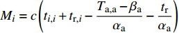
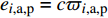
| cΔTi,a,p=αp(Mi+di,p−da,p+ei,a,p) | (19) |
where
Since the ordinary sensor node cannot initiatively send timestamps, the clock skew (i.e.,
| ΔT1,a,pΔTi,a,p=M1+d1,p−da,p+e1,a,pMi+di,p−da,p+ei,a,p,i∈{2,…,m}. | (20) |
Rearranging (20), one can obtain
| Qi,1,p+(1−Di,1,p)da,p=d1,p−Di,1,pdi,p+ei,1,p | (21) |
where
In order to minimize the measurement noise, we define
| minxpm∑i=2{[Qi,1,p+(1−Di,1,p)da,p−d1,p]2−(Di,1,pdi,p)2}2. | (22) |
The nonlinear problem in (22) can be transformed into the following linear LS problem
| minxp‖2Hxp−Q‖2 | (23) |
where
Remark 2: It is noticed that, at least five reference nodes are required to locate the ordinary sensor node
Accordingly, the direct estimation of
| ˆxp,direct=12(HTH)−1HTQ | (24) |
Similar to Section IV-A, the direct calculation of
| ˆxp,indirect=12˜H−1˜Q. | (25) |
With regard to (25), the main calculation process for ordinary sensor node is detailed as follows.
Step 1: Matrix Construction
For the convenience of computation, we define
| H11=m∑i=2[Di,1,p(pa−p1)+D2i,1,p(pi−pa)]×[Di,1,p(pa−p1)T+D2i,1,p(pi−pa)T]=(pa−p1)(pa−p1)Tm∑i=2D2i,1,p+(pa−p1)(−pTam∑i=2D3i,1,p+m∑i=2D3i,1,ppTi)+(−pam∑i=2D3i,1,p+m∑i=2D3i,1,ppi)(pa−p1)T |
| +m∑i=2D4i,1,ppapTa+m∑i=2D4i,1,ppipTi−m∑i=2D4i,1,ppipTa−pam∑i=2D4i,1,ppTiH12=m∑i=2[Di,1,p(pa−p1)+D2i,1,p(pi−pa)]×(1−Di,1,p)Qi,1,p=(pa−p1)m∑i=2(1−Di,1,p)Di,1,pQi,1,p−m∑i=2(1−Di,1,p)D2i,1,pQi,1,ppa+m∑i=2(1−Di,1,p)D2i,1,pQi,1,ppiH13=m∑i=2[Di,1,p(pa−p1)+D2i,1,p(pi−pa)](−Qi,1,p)=(pa−p1)m∑i=2(−Di,1,pQi,1,p)+m∑i=2D2i,1,p×Qi,1,ppa−m∑i=2D2i,1,pQi,1,ppiH21=HT12H31=HT13 |
| H22=m∑i=2(1−Di,1,p)2Q2i,1,pH23=−m∑i=2(1−Di,1,p)Q2i,1,pH32=−m∑i=2(1−Di,1,p)Q2i,1,pH33=m∑i=2Q2i,1,pQ11=m∑i=2[Di,1,p(pa−p1)+D2i,1,p(pi−pa)]×(−Q2i,1,p−(1−Di,1,p)2pTapa−pT1p1+2(1−Di,1,p)pTap1+D2i,1,ppTipi)=(pa−p1)m∑i=2(−Di,1,pQ2i,1,p)+(pam∑i=2D2i,1,pQ2i,1,p−m∑i=2D2i,1,pQ2i,1,ppi)+(pa−p1)(pTapa+pT1p1)×m∑i=2(−Di,1,p)+2(pa−p1)pTap1m∑i=2Di,1,p+(pam∑i=2D2i,1,p−m∑i=2D2i,1,ppi)(pTapa+pT1p1) |
| +2(pa−p1)pTa(pa−p1)m∑i=2D2i,1,p+2(−pa×m∑i=2D2i,1,p+m∑i=2D2i,1,ppi)pTap1+2(−pa×m∑i=2D3i,1,p+m∑i=2D3i,1,ppi)pTapa+(pa−p1)×(−pTapam∑i=2D3i,1,p+m∑i=2D3i,1,ppTipi)+2(pa×m∑i=2D3i,1,p−m∑i=2D3i,1,ppi)pTap1+(papTapa×m∑i=2D4i,1,p+m∑i=2D4i,1,ppipTipi)−m∑i=2D4i,1,ppipTapa−m∑i=2D4i,1,ppapTipi |
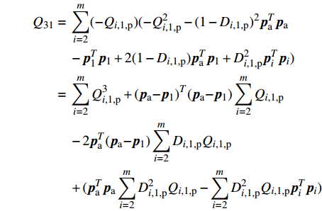
| Q31=m∑i=2(−Qi,1,p)(−Q2i,1,p−(1−Di,1,p)2pTapa−pT1p1+2(1−Di,1,p)pTap1+D2i,1,ppTipi)=m∑i=2Q3i,1,p+(pa−p1)T(pa−p1)m∑i=2Qi,1,p−2pTa(pa−p1)m∑i=2Di,1,pQi,1,p+(pTapam∑i=2D2i,1,pQi,1,p−m∑i=2D2i,1,pQi,1,ppTipi) |
| Q21=m∑i=2[(1−Di,1,p)Qi,1,p](−Q2i,1,p−(1−Di,1,p)2pTapa−pT1p1+2(1−Di,1,p)pTap1+D2i,1,ppTipi)=−m∑i=2(1−Di,1,p)Q3i,1,p−(pa−p1)T(pa−p1)×m∑i=2(1−Di,1,p)Qi,1,p+2pTa(pa−p1)×m∑i=2(1−Di,1,p)Di,1,pQi,1,p+(−pTapa×m∑i=2(1−Di,1,p)D2i,1,pQi,1,p+m∑i=2(1−Di,1,p)D2i,1,pQi,1,ppTipi). |
Therefore, the estimation of
| ˆxp,indirect=12[H11H12H13H21H22H23H31H32H33]−1[Q11Q21Q31]. | (26) |
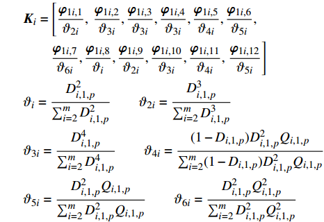
Step 2: PPS and PPDP Based State Calculation
Similar to Section IV-A, the real states of active sensor node are given as
In order to protect the privacy of
| \begin{split} & {{K}}_{i} = \left[\dfrac{{{\varphi }}_{1i,1}}{\vartheta _{2i}}, \right. \dfrac{{{\varphi }}_{1i,2}}{\vartheta _{3i}},\dfrac{{{\varphi }}_{1i,3}}{\vartheta _{3i}}, \dfrac{{{\varphi }}_{1i,4}}{\vartheta _{3i}}, \dfrac{{{\varphi }}_{1i,5}}{\vartheta _{4i}}, \dfrac{{{\varphi }}_{1i,6}}{\vartheta _{5i}}, \\&\quad\quad \dfrac{{{\varphi }}_{1i,7}}{\vartheta _{6i}}, \dfrac{{{\varphi }}_{1i,8}}{\vartheta _{i}}, \dfrac{{{\varphi }}_{1i,9}}{\vartheta _{2i}}, \dfrac{{{\varphi }}_{1i,10}}{\vartheta _{3i}}, \dfrac{{{\varphi }}_{1i,11}}{\vartheta _{4i}}, \left. \dfrac{{{\varphi }}_{1i,12}}{\vartheta _{5i}}\right]\\& \vartheta _{i} = \frac{D_{i,1,p}^{2}}{\sum\nolimits_{i = 2}^{m}D_{i,1,p}^{2}}\qquad\vartheta _{2i} = \frac{D_{i,1,p}^{3}}{\sum\nolimits_{i = 2}^{m}D_{i,1,p}^{3}} \\& \vartheta _{3i} = \frac{D_{i,1,p}^{4}}{\sum\nolimits_{i = 2}^{m}D_{i,1,p}^{4}}\qquad \vartheta _{4i} =\frac{(1-D_{i,1,p})D_{i,1,p}^{2}Q_{i,1,p}}{\sum\nolimits_{i = 2}^{m}(1-D_{i,1,p})D_{i,1,p}^{2}Q_{i,1,p}}\\& \vartheta _{5i} = \frac{D_{i,1,p}^{2}Q_{i,1,p}}{\sum\nolimits_{i = 2}^{m}D_{i,1,p}^{2}Q_{i,1,p}} \qquad \vartheta _{6i} = \frac{D_{i,1,p}^{2}Q_{i,1,p}^{2}}{\sum\nolimits_{i = 2}^{m}D_{i,1,p}^{2}Q_{i,1,p}^{2}} \end{split} |
for
With the similar strategy, the state

To protect the privacies of
Step 3: Calculation of
According to (26), the values of
Step 4: Position Estimation
Based on Step 3,
In the above sections, the proposed privacy preserving algorithms need cooperation among nodes, and require each node to be honest. However, underwater nodes are usually deployed in harsh and open environments, making them extremely vulnerable to security attack. For instance, an attacker can cause nodes to have imprecise locations, which leads to the dishonesty of nodes. To cope with this issue, we present the consequence when there exist dishonest nodes.
Without loss of generality, it is assumed that all the nodes are honest in the first localization interval, i.e.,
| {{p}}_{T_{\rm{a,a}}^{{\#}}} = {{p}}_{{\rm{a}}}+\delta \alpha _{{\rm{a}}}\sum\limits_{m_{{\rm{a}}} = 0}^{n_{{\rm{a}}}^{\#}}{{v}}_{{\rm{a}}}({\vec{T}}_{\rm{a,a}}). | (27) |
By employing the PPS-based localization algorithm in Section IV-A, the position of active sensor node at timestamp
Similarly, from (5), the position vector of ordinary sensor node at timestamp
| {{p}}_{T_{\rm{a,p}}^{{\#}}} = {{p}}_{{\rm{p}}}+\delta \alpha _{{\rm{p}}}\sum\limits_{m_{{\rm{p}}} = 0}^{n_{{\rm{p}}}^{\#}}{{v}}_{{\rm{p}}}({\vec{T}}_{\rm{a,p}}). | (28) |
With the PPS-based localization algorithm in Section IV-B, the position of ordinary sensor node at timestamp
In the following, let

We first investigate the equivalences of estimators (12) and (25). Then, the following theorems are given.
Theorem 1: Consider the linear LS problem for active sensor node, as described in (10). By applying the PPS-based asynchronous localization algorithm, the indirect estimation
Proof: It is noted that,
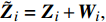
| \begin{split} & [{{A}}_{12},{{B}}_{12},(0;B_{21};0)] \\ & \quad ={\tilde{{Z}}}_{1}\sum\limits_{i = 2}^{m}{\rm{{\small diag}}}\{{\small \Upsilon }_{i,1},{\small \Upsilon }_{i,1}^{2},{\small \Upsilon }_{i,1}\} {\small +}\sum\limits_{i = 2}^{m}{\tilde{{Z}}}_{i}{\rm{{\small diag}}}\{ {\small \Upsilon }_{i,1},{\small \Upsilon }_{i,1}^{2},{\small \Upsilon }_{i,1}\} \\ & \quad={{Z}}_{1}\sum\limits_{i = 2}^{m}{\rm{{\small diag}}}\{{\small \Upsilon }_{i,1},{\small \Upsilon }_{i,1}^{2},{\small \Upsilon }_{i,1}\}{\small +}\sum\limits_{i = 2}^{m}{{Z}}_{i}{\rm{{\small diag}}}\{{\small \Upsilon }_{i,1},{\small \Upsilon }_{i,1}^{2},{\small \Upsilon }_{i,1}\} \\ & \quad \quad+{{\delta }}_{31}\sum\limits_{i = 2}^{m}{\rm{\small diag}}\{{\small \Upsilon }_{i,1},{\small \Upsilon }_{i,1}^{2},{\small \Upsilon }_{i,1}\}{\small +}\sum\limits_{i = 2}^{m}{{W}}_{i}{\rm{{\small diag}}}\{{\small \Upsilon }_{i,1},{\small \Upsilon }_{i,1}^{2},{\small \Upsilon }_{i,1}\}. \end{split} |
As
It is noticed that the values of
Theorem 2: Consider the linear LS problem for ordinary sensor node, as shown in (23). By applying PPS and PPDP based asynchronous localization algorithm, estimation
Proof: Referring to the elements of
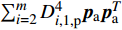
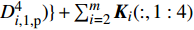
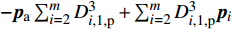
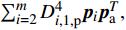
Next, we study the other elements of
| \begin{split} & \left[ \sum\limits_{i = 2}^{m}{\small D}_{i,1,{\rm{p}}}^{3}{{p}}_{i}{\small -}{{p}}_{{\rm{a}}}\sum\limits_{i = 2}^{m}{\small D}_{i,1,{\rm{p}}}^{3},\sum\limits_{i = 2}^{m}{\small D}_{i,1,{\rm{p}}}^{4}({{p}}_{\rm{a}}{{p}}_{{\rm{a}}}^{{T}}{\small +}{{p}}_{i}{{p}}_{i}^{{T}})\right] \\ & \quad = \tilde{{\bar{{X}}}}_{{\rm{a}}}(:,1{\small :}{4)\sum \limits_{i = 2}^{m}}{\rm{diag}}\{D_{i,1,{\rm{p}}}^{3},D_{i,1,{\rm{p}}}^{4},D_{i,1,{\rm{p}}}^{4},D_{i,1,{\rm{p}}}^{4}\} \\ &\quad\quad +\sum\limits_{i = 2}^{m}{\tilde{{\bar{{X}}}}_{i}(:,1{\small :}4)}{\rm{diag}}\{D_{i,1,{\rm{p}}}^{3},D_{i,1,{\rm{p}}}^{4},D_{i,1,{\rm{p}}}^{4},D_{i,1,{\rm{p}}}^{4}\} \\ & \quad = {\bar{{X}}}_{{\rm{a}}}(:,1{\small :}4){\sum\limits_{i = 2}^{m}}{\rm{diag}}\{D_{i,1,{\rm{p}}}^{3},D_{i,1,{\rm{p}}}^{4},D_{i,1,{\rm{p}}}^{4},D_{i,1,{\rm{p}}}^{4}\} \\ &\quad\quad +\sum\limits_{i = 2}^{m}{\bar{{X}}}_{i}(:,1{\small :}4){\rm{diag}}\{D_{i,1,{\rm{p}}}^{3},D_{i,1,{\rm{p}}}^{4},D_{i,1,{\rm{p}}}^{4},D_{i,1,{\rm{p}}}^{4}\} \\ &\quad\quad +{{\varphi }}_{1{\rm{a}}}(:,1{\small :}4){\sum\limits_{i = 2}^{m}}{\rm{diag}}\{D_{i,1,{\rm{p}}}^{3},D_{i,1,{\rm{p}}}^{4},D_{i,1,{\rm{p}}}^{4},D_{i,1,{\rm{p}}}^{4}\} \\ &\quad\quad +\sum\limits_{i = 2}^{m}{{K}}_{i}(:,1{\small :}4){\rm{diag}}\{D_{i,1,{\rm{p}}}^{3},D_{i,1,{\rm{p}}}^{4},D_{i,1,{\rm{p}}}^{4},D_{i,1,{\rm{p}}}^{4}\}.\end{split} |
It is noted that,
Based on this, we know
In the following, we investigate the level of privacy preservation for the proposed localization algorithms. To support our conclusion, the following definition is provided.
Definition 1 [19]: For node
Based on Definition 1, we have the following Theorem.
Theorem 3: With the LS estimator (12), the PPS-based asynchronous localization algorithm for active sensor node can guarantee the following levels of privacy preservation: 1) To anchor node
Proof: For anchor node 1, we have the values of
For anchor node
For active sensor node, the available information includes: range difference
In addition, we investigate the level of privacy preservation for the PPS and PPDP based localization algorithm.
Theorem 4: Consider the LS estimator (25), we have the following levels of privacy preservation: 1) To active sensor node, ordinary sensor node can preserve
Proof: For active sensor node, the location information of anchor node
For anchor node 2, we know the values of
For ordinary sensor node, the available information includes:
Corollary 1: Let us define
Proof: To start with, the time difference when anchor node
| \begin{split} & \Delta _{j,i} = t_{j,i}-t_{{\rm{a}},i},\;\;\;\;\;\;\Delta _{j,{\rm{p}}} = T_{j, {\rm{p}}}-T_{\rm{a,p}} \\ &\Delta _{i,{\rm{p}}} = T_{i,{\rm{p}}}-T_{j{\rm{,p}}},\;\Delta _{i, {\rm{a}}} = T_{i,{\rm{a}}}-T_{j{\rm{,a}}}. \end{split} | (29) |
From Fig. 2, one can infer that the conditions of preventing packet collision are
| \begin{split} &\Delta _{j,i} = \tau _{{\rm{a}},j}+(t_{j,j}-t_{{\rm{a}},j})+t_{{\rm{r,}}j}+\tau _{j,i}-\tau _{{\rm{a,}}i}>0 \\ &\Delta _{j,{\rm{p}}} = \tau _{{\rm{a}},j}+(t_{j,j}-t_{{\rm{a}},j})+t_{{\rm{r,}}j}+\tau _{j,{\rm{p}}}-\tau _{\rm{a,p}}>0 \\ &\Delta _{i,{\rm{p}}} = \tau _{j,i}+(t_{i,i}-t_{j,i})+t_{{\rm{r,}}i}+\tau _{i,{\rm{p}}}-\tau _{j,{\rm{p}}}>0 \\ &\Delta _{i,{\rm{a}}} = \tau _{j,i}+(t_{i,i}-t_{j,i})+t_{{\rm{r,}}i}+\tau _{{\rm{a}},i}-\tau _{{\rm{a}},j}>0 \end{split} | (30) |
which yields
| \begin{split} & t_{j,j}-t_{{\rm{a}},j} >\dfrac{(d_{{\rm{a}},i}-d_{{\rm{a}},j}-d_{j,i})}{c}-t_{{\rm{r,}}j} \\ & t_{j,j}-t_{{\rm{a}},j} >\dfrac{(d_{\rm{a,p}}-d_{{\rm{a}},j}-d_{j,{\rm{p}}})}{c}-t_{{\rm{r}},j} \\ & t_{i,i}-t_{j,i} >\dfrac{(d_{j{\rm{,p}}}-d_{j,i}-d_{i{\rm{,p}}})}{c}-t_{{\rm{r}},i}\\ &t_{i,i}-t_{j,i} >\dfrac{(d_{{\rm{a}},j}-d_{j,i}-d_{{\rm{a,}}i})}{c}-t_{{\rm{r}},i}. \end{split} | (31) |
Clearly, if
In this section, we analyse the communication overhead of the proposed localization algorithms. Referring to [18], one knows the communication overhead is evaluated by the transmission of elements. Meanwhile, it is easy to see that the communication overhead of PPS-based localization algorithm for active sensor node is dominated by the state calculation in Step 2. Similarly, the communication overhead of PPS and PPDP based localization algorithm for ordinary sensor node is also dominated by the state calculation in Step 2. Accordingly, the transmission of elements of localization algorithm for active sensor node can be calculated as
| \begin{split} &\begin{array}{c} \Psi _{{\rm{a}}} = \underbrace{ \ 6(m-1)(m-2)+6(m-1)\ } \\ {{{\rm{\rm{\; elements \;of \;calculating}}}\sum\limits_{i = 2}^{m}{{X}}_{i}}}\end{array} \\ & \quad\quad\begin{array}{c}+ \underbrace{{ \ \ \ }12m(m-1)+12m \ \ \ \ } \\ {{{\rm{\rm{\; elements \;of \;calculating}}}\sum\limits_{i = 1}^{m}{{Y}}_{i}}}\end{array} \\ & \quad\quad\begin{array}{c}+ \underbrace{ \ 2(m-1)+9m(m-1)+9m \ } \\ {{{\rm{\rm{\; elements \;of \;calculating}}}\ {{Z}}_{i}}}\end{array} \\ &\quad= 27m^{2}-10m+4. \end{split} | (32) |
Similarly, the transmission of elements of localization algorithm for ordinary sensor node can be calculated as
| \begin{split} & \begin{array}{c}\Psi _{{\rm{p}}} = \underbrace{ \ 36m(m-1)+6(m-1)+36m \ } \\ {{{\rm{\;elements \;of \;calculating}} \;{\bar{{X}}}_{{\rm{a}}}\;{ \rm{\small\;and} }\;{\bar{{X}}}_{i}}}\end{array} \\ & \quad \begin{array}{c}+ \underbrace{{ \ \ \ \ \ \ \ }6\times 2+6\times 2{ \ \ \ \ \ \ \ \ }} \\ {{{\rm{\;elements \;of \;calculating }}\;{\bar{{Y}}}_{{\rm{a}}}\;{\rm {and}} \;{\bar{{Y}}}_{1}}}\end{array} \\ & \quad\quad \begin{array}{c}+ \underbrace{{ \ \ \ }15(m-1)+15(m-1)+9 \ } \\ {{{\rm{\;elements \;of \;calculating}}\;{\tilde{{\bar{{Z}}}}_{i}}{\bar{{Z}}}_{{\rm{a}}}}}\end{array} \\ & \quad\;\; \begin{array}{c}+ \underbrace{{ \ \ \ \ \ \ \ \ }3\times 3\times 3{ \ \ \ \ \ \ \ \ \ \ \ \ }} \\ {{{\rm{\rm{\small\; elements \;of\; calculating}}}{{\ }}{\bar{{M}}}_{{\rm{a}}}{\bar{{M}}}_{1}}}\end{array} \\ & \quad\;\; \begin{array}{c}+ \underbrace{{ \ \ \ \ \ \ \ \ }3\times 3\times 3{ \ \ \ \ \ \ \ \ \ \ \ \ }} \\ {{{\rm{\;elements\; of \;calculating}}{{\ }}{\bar{{M}}}_{{\rm{a}}}{\bar{{M}}}_{2}}}\end{array} \\ &\quad = 36m^{2}+36m+51. \end{split} | (33) |
In this section, the simulations are implemented on MATLAB 2017b. Initially, ten active sensor nodes and ten ordinary sensor nodes are randomly deployed in an area of

1) Equivalence Between Our Method and Traditional Method
It is noted that, the privacy preservation is employed into the asynchronous localization of USNs, through which PPS and PPDP based localization algorithms are designed to hide privacy information. To verify the effectiveness of the proposed localization algorithms, the actual and localized positions of active sensor node (labelled as “1”) are shown in Fig. 8(a). In this figure, the traditional LS method refers to the estimation in (11), where the privacy preservation of anchor nodes is not considered. For clear description, the localization error of active sensor node is defined as err

Similarly, the actual and localized positions of ordinary sensor node (labelled as “2”) are also shown in Fig. 8(a). Define the localization error of ordinary sensor node as err
2) Comparison With Synchronous Localization Algorithm
In [19], the authors adopted PPS into TDOA-based localization, where the target sends localization request to anchor nodes. However, the TDOA-based localization method in [19] can achieve localization task only in the case of synchronized clock, i.e.,

3) Comparison With Asynchronous Localization Algorithm
To remove the influence of asynchronous clocks, an asynchronous localization algorithm based on iterative least squares estimators was presented in [13], where the clock skew was ignored, i.e.,

4) Performance for the Mobility Compensation Strategy
As provided in Section III-B, a mobility compensation strategy is developed to balance the tradeoff between communication cost and localization accuracy. To verify the effectiveness, the measurement window

5) Consequence When There Exist Dishonest Nodes
In the above results, the nodes are assumed to be honest. As mentioned in Section IV-C, if the condition of

Experiment results are presented in this section, and we only check the effectiveness of the PPS-based asynchronous localization algorithm for active sensor node due to limited experiment conditions in our lab. To be specific, the experiment is carried out in a tank of
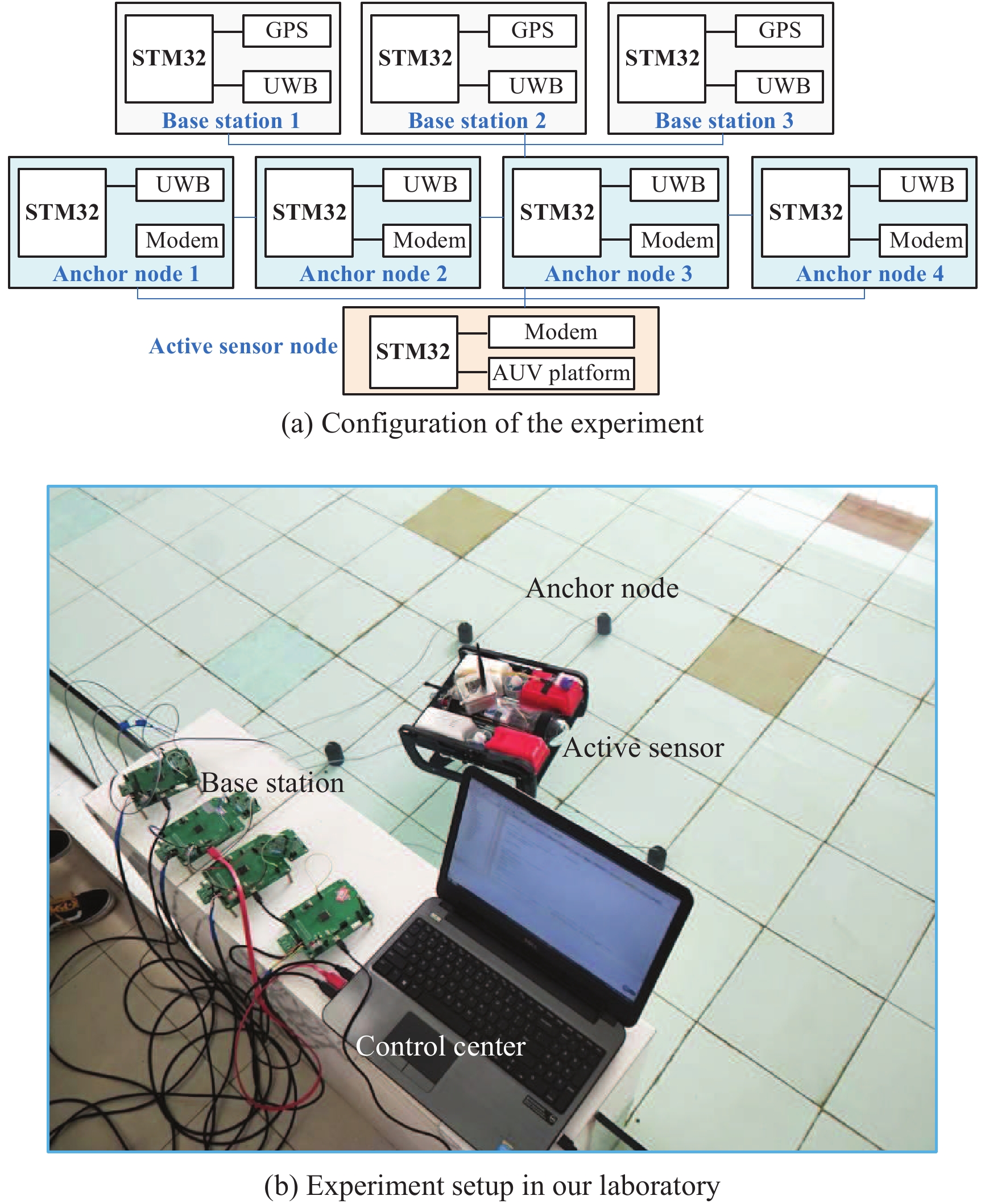
In order to estimate the position of active sensor node, underwater acoustic modems are required to provide communication capability for the sensor-to-anchor wireless links. Then, an acoustic modem that consists of STM32 processor, transmitter and receiver is designed in our lab, as shown in Fig. 14(a). To verify the effectiveness of our modem, the received analog signals are presented on the top of Fig. 14(b). These analog signals can be converted to digital signals, as shown on the bottom of Fig. 14(b). Clearly, the transmitted preamble and the guard interval in Fig. 14 can be identified, which indirectly verify the effectiveness of the designed acoustic modem.

With the embedded communication system, the position of active sensor node can be estimated. To this end, the position vectors of anchor nodes are set as
| T_{\rm{a,a}} | t_{\rm{a,1}} | t_{\rm{a,2}} | t_{\rm{a,3}} | t_{\rm{a,4}} | |
| Point 1 | 64 762 | 65 584 | 65 892 | 65 582 | 65 042 |
| Point 2 | 65 637 | 66 530 | 66 637 | 66 270 | 66 084 |
| Point 3 | 62 384 | 63 104 | 63 233 | 63 104 | 62 949 |
| Point 4 | 72 563 | 73 129 | 73 283 | 73 412 | 73 284 |
| Point 5 | 84 369 | 84 816 | 85 002 | 85 369 | 85 263 |
| Point 6 | 57 296 | 57 929 | 57 743 | 58 190 | 58 296 |
| Point 7 | 66 437 | 67 257 | 66 717 | 67 257 | 67 567 |
| Point 8 | 82 653 | 83 547 | 83 100 | 83 286 | 83 653 |
| Point 9 | 54 698 | 55 698 | 55 331 | 55 145 | 55 592 |
| Point 10 | 72 734 | 73 864 | 73 554 | 73 014 | 73 558 |
| Point 11 | 63 647 | 64 927 | 64 447 | 63 847 | 64 667 |
DownLoad:
CSV

With consideration of privacy preservation, this paper studies an asynchronous localization issue for USNs. In order to eliminate the effect of asynchronous clocks (i.e., clock offset and skew), an asynchronous localization protocol including mobility compensation strategy is presented. Based on this, the PPS and PPDP based localization algorithms are designed to hide privacy information, where the performance analyses are also presented. Finally, simulation and experiment results show that the localization algorithm in this paper can achieve localization task, while the effect of clock can be eliminated.
| [1] |
J. Yan, Y. D. Gong, C. L. Chen, X. Y. Luo, and X. P. Guan, “AUV-aided localization for internet of underwater things: A reinforcement learningbased method,” IEEE Internet Things J., 2020, DOI: 10.1109/JIOT.2020.2993012.
|
| [2] |
J. Yan, H. Y. Zhao, X. Y. Luo, C. L. Chen, and X. P. Guan, “RSSI-based heading control for robust long-range aerial communication in UAV networks,” IEEE Internet Things J., vol. 6, no. 2, pp. 1675–1689, Apr. 2019. doi: 10.1109/JIOT.2018.2875428
|
| [3] |
S. M. Jiang, “On reliable data transfer in underwater acoustic networks: A survey from networking perspective,” IEEE Commun. Surv. and Tutorials, vol. 20, no. 2, pp. 1036–1055, May 2018.
|
| [4] |
J. Yan, D. B. Guo, X. Y. Luo, and X. P. Guan, “AUV-aided localization for underwater acoustic sensor networks with current field estimation,” IEEE Trans. Veh. Technol., 2020, DOI: 10.1109/TVT.2020.2996513.
|
| [5] |
D. Zhang, M. Q. Liu, S. L. Zhang, and Q. F. Zhang, “Non-myopic energy allocation for target tracking in energy harvesting UWSNs,” IEEE Sens. J., vol. 19, no. 10, pp. 3772–3783, May 2019. doi: 10.1109/JSEN.2018.2890078
|
| [6] |
Z. Y. Gao, and G. Guo, “Fixed-time sliding mode formation control of AUVs based on a disturbance observer,” IEEE/CAA J. Autom. Sinica, vol. 7, no. 2, pp. 539–545, Mar. 2020. doi: 10.1109/JAS.2020.1003057
|
| [7] |
S. Wang, L. Chen, D. B. Gu, and H. S. Hu, “Cooperative localization of AUVs using moving horizon estimation,” IEEE/CAA J. Autom. Sinica, vol. 1, no. 1, pp. 68–76, Jan. 2014. doi: 10.1109/JAS.2014.7004622
|
| [8] |
J. Wang, X. Zhang, Q. H. Gao, H. Yue, and H. Y. Wang, “Device-free wireless localization and activity recognition: A deep learning approach,” IEEE Trans. Veh. Technol., vol. 66, no. 7, pp. 6258–6267, Jul. 2017. doi: 10.1109/TVT.2016.2635161
|
| [9] |
G. J. Han, X. Yang, L. Liu, W. B. Zhang, and M. Guizani, “A disaster management-oriented path planning for mobile anchor node-based localization in wireless sensor networks,” IEEE Trans. Emerg. Top. Comput., vol. 8, no. 1, pp. 115–125, Jan. 2020. doi: 10.1109/TETC.2017.2687319
|
| [10] |
J. Wang, L. M. Zhang, Q. H. Gao, M. Pan, and H. Y. Wang, “Device-free wireless sensing in complex scenarios using spatial structural information,” IEEE Trans. Wireless Commun., vol. 17, no. 4, pp. 2432–2442, Apr. 2018. doi: 10.1109/TWC.2018.2796086
|
| [11] |
B. W. Chen, S. Rho, M. Imran, M. Guizani, and W. K. Fan, “Cognitive sensors based on ridge phase-smoothing localization and multiregional histograms of oriented gradients,” IEEE Trans. Emerg. Top. Comput., vol. 7, no. 1, pp. 123–134, Mar. 2019. doi: 10.1109/TETC.2016.2585040
|
| [12] |
P. Carroll, K. Mahmood, S. L. Zhou, H. Zhou, X. K. Xu, and J. W. Cui, “Ondemand asynchronous localization for underwater sensor networks,” IEEE Trans. Signal Process., vol. 62, no. 13, pp. 3337–3348, Jul. 2014. doi: 10.1109/TSP.2014.2326996
|
| [13] |
J. Yan, X. N. Zhang, X. Y. Luo, Y. Y. Wang, C. L. Chen, and X. P. Guan, “Asynchronous localization with mobility prediction for underwater acoustic sensor networks,” IEEE Trans. Veh. Technol., vol. 67, no. 3, pp. 2543–2556, Mar. 2018. doi: 10.1109/TVT.2017.2764265
|
| [14] |
J. Liu, Z. H. Wang, J. H. Cui, S. L. Zhou, and B. Yang, “A joint time synchronization and localization design for mobile underwater sensor networks,” IEEE Trans. Mob. Comput., vol. 15, no. 3, pp. 530–543, Mar. 2016. doi: 10.1109/TMC.2015.2410777
|
| [15] |
E. Mortazavi, R. Javidan, M. Dehghani, and V. Kavoosi, “A robust method for underwater wireless sensor joint localization and synchronization,” Ocean Eng., vol. 137, no. 2, pp. 276–286, Jun. 2017.
|
| [16] |
H. Li, Y. H. He, X. Z. Cheng, H. S. Zhu, and L. M. Sun, “Security and privacy in localization for underwater sensor networks,” IEEE Commun. Mag., vol. 53, no. 11, pp. 56–62, Nov. 2015. doi: 10.1109/MCOM.2015.7321972
|
| [17] |
A. Konstantinidis, G. Chatzimilioudis, D. Zeinalipour-Yazti, P. Mpeis, N. Pelekis, and Y. Theodoridis, “Privacy-preserving indoor localization on smartphones,” IEEE Trans. Knowl. Data Eng., vol. 27, no. 11, pp. 3042–3055, Nov. 2015. doi: 10.1109/TKDE.2015.2441724
|
| [18] |
T. Shu, Y. Y. Chen, and J. Yang, “Protecting multi-lateral privacy in pervasive environments,” IEEE/ACM Trans. Netw., vol. 23, no. 5, pp. 1688–1701, Oct. 2015. doi: 10.1109/TNET.2015.2478881
|
| [19] |
X. F. Shi and J. F. Wu, “To hide private position information in localization using time difference of arrival,” IEEE Trans. Signal Process., vol. 66, no. 18, pp. 4946–4956, Sep. 2018. doi: 10.1109/TSP.2018.2858187
|
| [20] |
G. H. Wang, J. P. He, X. F. Shi, J. P. Pan, and S. B. Shen, “Analyzing and evaluating efficient privacy-preserving localization for pervasive computing,” IEEE Internet Things J., vol. 5, no. 4, pp. 2993–3007, Aug. 2018. doi: 10.1109/JIOT.2017.2772291
|
| [21] |
X. Z. Cheng, H. N. Shu, Q. L. Liang, and D. H. C. Du, “Silent positioning in underwater acoustic sensor networks,” IEEE Trans. Veh. Technol., vol. 57, no. 3, pp. 1756–1766, May 2008. doi: 10.1109/TVT.2007.912142
|
| [22] |
X. Liu, J. J. Yin, S. G. Zhang, B. Ding, S. Guo, and K. Wang, “Range-based localization for sparse 3-D sensor networks,” IEEE Internet Things J., vol. 6, no. 1, pp. 753–764, Feb. 2019. doi: 10.1109/JIOT.2018.2856267
|
| [23] |
J. M. Chen, C. Q. Wang, Y. X. Sun, and X. M. Shen, “Semi-supervised laplacian regularized least squares algorithm for localization in wireless sensor networks,” Comput. Netw., vol. 55, no. 10, pp. 2481–2491, Apr. 2011. doi: 10.1016/j.comnet.2011.04.010
|
| [24] |
F. Zafari, A. Gkelias, and K. K. Leung, “A survey of indoor localization systems and technologies,” IEEE Commun. Surv. and Tutorials, vol. 21, no. 3, pp. 2568–2599, Apr. 2019.
|
| [25] |
P. H. Tsai, R. G. Tsai, and S. S. Wang, “Hybrid localization approach for underwater sensor networks,” J. Sensors, vol. 2017, no. 2017, pp. 1–13, Nov. 2017.
|
| [26] |
Z. Zhou, Z. Peng, J. H. Cui, Z. J. Shi, and A. Bagtzoglou, “Scalable localization with mobility prediction for underwater sensor networks,” IEEE Trans. Mob. Comput., vol. 10, no. 3, pp. 335–348, Mar. 2011. doi: 10.1109/TMC.2010.158
|
| [27] |
B. B. Zhang, H. Y. Wang, L. M. Zheng, J. F. Wu, and Z. W. Zhuang, “Joint synchronization and localization for underwater sensor networks considering stratification effect,” IEEE Access, vol. 5, no. 1, pp. 26932–26943, Nov. 2017.
|
| [28] |
Z. J. Gong, C. Li, and F. Jiang, “AUV-aided joint localization and time synchronization for underwater acoustic sensor networks,” IEEE Signal Process. Lett., vol. 25, no. 4, pp. 477–481, Apr. 2018. doi: 10.1109/LSP.2018.2799699
|
| [29] |
J. Yan, H. J. Ban, X. Y. Luo, H, Y. Zhao, and X. P. Guan, “Joint localization and tracking design for AUV with asynchronous clocks and state disturbances,” IEEE Trans. Veh. Technol., vol. 68, no. 5, pp. 4707–4720, Mar. 2019. doi: 10.1109/TVT.2019.2903212
|
| [30] |
J. Yan, H. Y. Zhao, Y. Y. Wang, X. Y. Luo, and X. P. Guan, “Asynchronous localization for UASNs: An unscented transform-based method,” IEEE Signal Process. Lett., vol. 26, no. 4, pp. 602–606, Apr. 2019. doi: 10.1109/LSP.2019.2902273
|
| [31] |
T. Alexandri, E. Miller, E. Spanier, and R. Diamant, “Tracking the slipper lobster using acoustic tagging: Testbed description,” IEEE J. Oceanic Eng., vol. 45, no. 2, pp. 577–585, Apr. 2020. doi: 10.1109/JOE.2018.2880862
|
| [32] |
D. Haddad, W. Martins, M. Costa, L. Biscainho, L. Nunes, and B. Lee, “Robust acoustic self-localization of mobile devices,” IEEE Trans. Mob. Comput., vol. 15, no. 4, pp. 982–995, Apr. 2016. doi: 10.1109/TMC.2015.2439278
|
| [33] |
R. Diamant and L. Lampe, “Underwater localization with timesynchronization and propagation speed uncertainties,” IEEE Trans. Mob. Comput., vol. 12, no. 7, pp. 1257–1269, Jul. 2013. doi: 10.1109/TMC.2012.100
|
| [34] |
A. Jolfaei, X. W. Wu, and V. Muthukkumarasamy, “On the security of permutation-only image encryption schemes,” IEEE Trans. Inf. Forensics Secur., vol. 11, no. 2, pp. 235–246, Feb. 2016. doi: 10.1109/TIFS.2015.2489178
|
| [35] |
P. Ostovari, J. Wu, A. Khreishah, and N. B. Shroff, “Scalable video streaming with helper nodes using random linear network coding,” IEEE/ACM Trans. Netw., vol. 24, no. 3, pp. 1574–1587, Jun. 2016. doi: 10.1109/TNET.2015.2427161
|
| [36] |
M. Aiash, R. Colson, and M. Kallash, “Introducing a hybrid infrastructure and information-centric approach for secure cloud computing,” in Proc. IEEE Int. Conf. Advanced Information Networking and Applications, Gwangiu, South Korea, Feb. 2015, 154−159.
|
| [37] |
S. W. Wang, L. S. Huang, Y. W. Nie, P. Z. Wang, H. L. Xu, and W. Yang, “PrivSet: Set-valued data analyses with locale differential privacy,” in Proc. IEEE INFOCOM, Honolulu, USA, Apr. 2018, 1088−1096.
|
| [38] |
Y. F. Wang, M. J. Huang, Q. Jin, and J. H. Ma, “DP3: A differential privacybased privacy-preserving indoor localization mechanism,” IEEE Commun. Lett., vol. 22, no. 12, pp. 2547–2550, Dec. 2018. doi: 10.1109/LCOMM.2018.2876449
|
| [39] |
J. Liu, Z. H. Wang, Z. Peng, J. H. Cui, and L. Fiondella, “Suave: Swarm underwater autonomous vehicle localization,” in Proc. IEEE INFOCOM, Toronto, Canada, Apr. 2014, 64−72.
|
| [40] |
C. Bechaz and H. Thomas, “GIB system: The underwater GPS solution,” in Proc. 5th ECUA, Villeurbanne, May 2000, 613−618.
|
| [41] |
G. Aiello and G. Rogerson, “Ultra-wideband wireless systems,” IEEE Microwave Mag., vol. 4, no. 2, pp. 36–47, Jun. 2003. doi: 10.1109/MMW.2003.1201597
|
| [1] | Mengli Wei, Wenwu Yu, Duxin Chen, Mingyu Kang, Guang Cheng. Privacy Distributed Constrained Optimization Over Time-Varying Unbalanced Networks and Its Application in Federated Learning[J]. IEEE/CAA Journal of Automatica Sinica, 2025, 12(2): 335-346. doi: 10.1109/JAS.2024.124869 |
| [2] | Zhongyuan Zhao, Zhiqiang Yang, Luyao Jiang, Ju Yang, Quanbo Ge. Privacy Preserving Distributed Bandit Residual Feedback Online Optimization Over Time-Varying Unbalanced Graphs[J]. IEEE/CAA Journal of Automatica Sinica, 2024, 11(11): 2284-2297. doi: 10.1109/JAS.2024.124656 |
| [3] | Minfeng Qi, Ziyuan Wang, Qing-Long Han, Jun Zhang, Shiping Chen, Yang Xiang. Privacy Protection for Blockchain-Based Healthcare IoT Systems: A Survey[J]. IEEE/CAA Journal of Automatica Sinica, 2024, 11(8): 1757-1776. doi: 10.1109/JAS.2022.106058 |
| [4] | Zheng Wu, Yiyun Zhao, Fanbiao Li, Tao Yang, Yang Shi, Weihua Gui. Asynchronous Learning-Based Output Feedback Sliding Mode Control for Semi-Markov Jump Systems: A Descriptor Approach[J]. IEEE/CAA Journal of Automatica Sinica, 2024, 11(6): 1358-1369. doi: 10.1109/JAS.2024.124416 |
| [5] | Xuerao Wang, Qingling Wang, Yanxu Su, Yuncheng Ouyang, Changyin Sun. Adaptive Sensor-Fault Tolerant Control of Unmanned Underwater Vehicles With Input Saturation[J]. IEEE/CAA Journal of Automatica Sinica, 2024, 11(4): 907-918. doi: 10.1109/JAS.2023.123837 |
| [6] | Wei Chen, Guo-Ping Liu. Privacy-Preserving Consensus-Based Distributed Economic Dispatch of Smart Grids via State Decomposition[J]. IEEE/CAA Journal of Automatica Sinica, 2024, 11(5): 1250-1261. doi: 10.1109/JAS.2023.124122 |
| [7] | Meiqin Tang, Jiawen Sheng, Shaoyan Sun. A Coverage Optimization Algorithm for Underwater Acoustic Sensor Networks based on Dijkstra Method[J]. IEEE/CAA Journal of Automatica Sinica, 2023, 10(8): 1769-1771. doi: 10.1109/JAS.2023.123279 |
| [8] | Feiye Zhang, Qingyu Yang, Dou An. Privacy Preserving Demand Side Management Method via Multi-Agent Reinforcement Learning[J]. IEEE/CAA Journal of Automatica Sinica, 2023, 10(10): 1984-1999. doi: 10.1109/JAS.2023.123321 |
| [9] | Zijun Gong, Cheng Li, Ruoyu Su. Fundamental Limits of Doppler Shift-Based, ToA-Based, and TDoA-Based Underwater Localization[J]. IEEE/CAA Journal of Automatica Sinica, 2023, 10(7): 1637-1639. doi: 10.1109/JAS.2023.123282 |
| [10] | Wenchao Huang, Zhijun Pan, Zhezhuang Xu. Underwater Cable Localization Method Based on Beetle Swarm Optimization Algorithm[J]. IEEE/CAA Journal of Automatica Sinica, 2023, 10(9): 1893-1895. doi: 10.1109/JAS.2022.106073 |
| [11] | Ya Wang, Xinming Chen, Lei Shi, Yuhua Cheng, Houjun Wang. A Trust Assessment-Based Distributed Localization Algorithm for Sensor Networks Under Deception Attacks[J]. IEEE/CAA Journal of Automatica Sinica, 2022, 9(10): 1879-1882. doi: 10.1109/JAS.2022.105881 |
| [12] | Yifan Xia, Hui Yu, Fei-Yue Wang. Accurate and Robust Eye Center Localization via Fully Convolutional Networks[J]. IEEE/CAA Journal of Automatica Sinica, 2019, 6(5): 1127-1138. doi: 10.1109/JAS.2019.1911684 |
| [13] | Zhen Hong, Rui Wang, Xile Li. A Clustering-tree Topology Control Based on the Energy Forecast for Heterogeneous Wireless Sensor Networks[J]. IEEE/CAA Journal of Automatica Sinica, 2016, 3(1): 68-77. |
| [14] | Zhaolei Wang, Qing Wang, Chaoyang Dong. Asynchronous H∞ Control for Unmanned Aerial Vehicles: Switched Polytopic System Approach[J]. IEEE/CAA Journal of Automatica Sinica, 2015, 2(2): 207-216. |
| [15] | Changqing Xia, Wei Liu, Qingxu Deng. Cost Minimization of Wireless Sensor Networks with Unlimited-lifetime Energy for Monitoring Oil Pipelines[J]. IEEE/CAA Journal of Automatica Sinica, 2015, 2(3): 290-295. |
| [16] | Zhixin Liu, Yazhou Yuan, Xinping Guan, Xinbin Li. An Approach of Distributed Joint Optimization for Cluster-based Wireless Sensor Networks[J]. IEEE/CAA Journal of Automatica Sinica, 2015, 2(3): 267-273. |
| [17] | Xiaoyuan Luo, Liu Feng, Jing Yan, Xinping Guan. Dynamic Coverage with Wireless Sensor and Actor Networks in Underwater Environment[J]. IEEE/CAA Journal of Automatica Sinica, 2015, 2(3): 274-281. |
| [18] | Haiyang Yu, Yisha Liu, Wei Wang. Distributed Sparse Signal Estimation in Sensor Networks Using H∞-Consensus Filtering[J]. IEEE/CAA Journal of Automatica Sinica, 2014, 1(2): 149-154. |
| [19] | Yi Dong, Jie Huang. Leader-following Rendezvous with Connectivity Preservation of Single-integrator Multi-agent Systems[J]. IEEE/CAA Journal of Automatica Sinica, 2014, 1(1): 19-23. |
| [20] | Sen Wang, Ling Chen, Dongbing Gu, Huosheng Hu. Cooperative Localization of AUVs Using Moving Horizon Estimation[J]. IEEE/CAA Journal of Automatica Sinica, 2014, 1(1): 68-76. |

Figures(15) / Tables(2)


Haiyan Zhao, Jing Yan, Xiaoyuan Luo and Xinping Guan, "Privacy Preserving Solution for the Asynchronous Localization of Underwater Sensor Networks," IEEE/CAA J. Autom. Sinica, vol. 7, no. 6, pp. 1511-1527, Nov. 2020. doi: 10.1109/JAS.2020.1003312
| Notation | Description | |
| T_{\rm{a,a}} | Time when active sensor sends initiator message | |
| t_{{\rm{a}},i} | Time when anchor i receives initiator message | |
| t_{i,i} | Time when anchor i sends message | |
| t_{j,i} | Time when anchor i receives message from anchor j | |
| T_{i,{\rm{a}}} | Time when active sensor receives message from anchor i | |
| T_{\rm{a,p}} | Time when ordinary sensor receives message from active sensor | |
| T_{i,{\rm{p}}} | Time when ordinary sensor receives message from anchor i | |
| \varpi _{i,1} | Time measurement noise between anchor i and anchor 1 | |
| \varpi _{i,{\rm{p}}} | Time measurement noise between anchor i and ordinary sensor |
DownLoad:
CSV
| T_{\rm{a,a}} | t_{\rm{a,1}} | t_{\rm{a,2}} | t_{\rm{a,3}} | t_{\rm{a,4}} | |
| Point 1 | 64 762 | 65 584 | 65 892 | 65 582 | 65 042 |
| Point 2 | 65 637 | 66 530 | 66 637 | 66 270 | 66 084 |
| Point 3 | 62 384 | 63 104 | 63 233 | 63 104 | 62 949 |
| Point 4 | 72 563 | 73 129 | 73 283 | 73 412 | 73 284 |
| Point 5 | 84 369 | 84 816 | 85 002 | 85 369 | 85 263 |
| Point 6 | 57 296 | 57 929 | 57 743 | 58 190 | 58 296 |
| Point 7 | 66 437 | 67 257 | 66 717 | 67 257 | 67 567 |
| Point 8 | 82 653 | 83 547 | 83 100 | 83 286 | 83 653 |
| Point 9 | 54 698 | 55 698 | 55 331 | 55 145 | 55 592 |
| Point 10 | 72 734 | 73 864 | 73 554 | 73 014 | 73 558 |
| Point 11 | 63 647 | 64 927 | 64 447 | 63 847 | 64 667 |
DownLoad:
CSV
| Notation | Description | |
| T_{\rm{a,a}} | Time when active sensor sends initiator message | |
| t_{{\rm{a}},i} | Time when anchor i receives initiator message | |
| t_{i,i} | Time when anchor i sends message | |
| t_{j,i} | Time when anchor i receives message from anchor j | |
| T_{i,{\rm{a}}} | Time when active sensor receives message from anchor i | |
| T_{\rm{a,p}} | Time when ordinary sensor receives message from active sensor | |
| T_{i,{\rm{p}}} | Time when ordinary sensor receives message from anchor i | |
| \varpi _{i,1} | Time measurement noise between anchor i and anchor 1 | |
| \varpi _{i,{\rm{p}}} | Time measurement noise between anchor i and ordinary sensor |
| T_{\rm{a,a}} | t_{\rm{a,1}} | t_{\rm{a,2}} | t_{\rm{a,3}} | t_{\rm{a,4}} | |
| Point 1 | 64 762 | 65 584 | 65 892 | 65 582 | 65 042 |
| Point 2 | 65 637 | 66 530 | 66 637 | 66 270 | 66 084 |
| Point 3 | 62 384 | 63 104 | 63 233 | 63 104 | 62 949 |
| Point 4 | 72 563 | 73 129 | 73 283 | 73 412 | 73 284 |
| Point 5 | 84 369 | 84 816 | 85 002 | 85 369 | 85 263 |
| Point 6 | 57 296 | 57 929 | 57 743 | 58 190 | 58 296 |
| Point 7 | 66 437 | 67 257 | 66 717 | 67 257 | 67 567 |
| Point 8 | 82 653 | 83 547 | 83 100 | 83 286 | 83 653 |
| Point 9 | 54 698 | 55 698 | 55 331 | 55 145 | 55 592 |
| Point 10 | 72 734 | 73 864 | 73 554 | 73 014 | 73 558 |
| Point 11 | 63 647 | 64 927 | 64 447 | 63 847 | 64 667 |
 DownLoad:


 DownLoad:


