Figure
1.
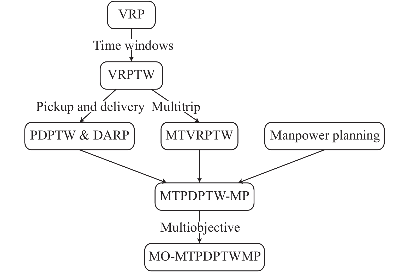
Relationship between MO-MTPDPTWMP and various VRP extensions. The problem highlighted in bold is studied in this paper.
 Volume 7
Issue 4
Volume 7
Issue 4
IEEE/CAA Journal of Automatica Sinica
| Citation: | Jiahai Wang, Yuyan Sun, Zizhen Zhang and Shangce Gao, "Solving Multitrip Pickup and Delivery Problem With Time Windows and Manpower Planning Using Multiobjective Algorithms," IEEE/CAA J. Autom. Sinica, vol. 7, no. 4, pp. 1134-1153, July 2020. doi: 10.1109/JAS.2020.1003204

|
THE vehicle routing problem (VRP) can be described as the problem of designing an optimal set of routes such that all the customers’ requirements and the operational constraints are satisfied. The VRP has direct applications to everyday business routines of distribution or service-providing companies. A broad range of possible extensions to the VRP formulation are covered in [1]–[5]. Most research focuses on a widely used variant, called VRP with time windows (VRPTW). Thereafter, further extensions of the VRPTW, such as the pickup and delivery problem with time windows (PDPTW), the dial-a-ride problem (DARP) and the multitrip VRP with time windows (MTVRPTW), were proposed [6]–[8]. Besides, some research considers integrating the manpower planning into VRP since the driving of vehicles and the provision of services require the participation of manpower [9]. Recently, a more practical variant, called multitrip pickup and delivery problem with time windows and manpower planning (MTPDPTW-MP) was introduced in [9]. Relationship between this problem and other VRP extensions mentioned above is shown in Fig. 1.
MTPDPTW-MP is a real-life healthcare problem originated from the application of Hong Kong public hospitals, China. Transportation services are provided to disabled or elderly patients between their residences and clinics. The ambulance routes satisfying a series of constraints should be designed and the staff assignment is also required [10], [11]. MTPDPTW-MP is an NP-hard problem of high complexity, as it is a combination of two well-known NP-hard problems (i.e., PDPTW and the staff scheduling problem). Usually, metaheuristic search techniques [12] are used to solve this kind of problems. In [9], an iterated local search (ILS) metaheuristic using a variable neighborhood descent (VND) procedure in the local search phase, called ILS-VND, was proposed to deal with MTPDPTW-MP. [9] considered MTPDPTW-MP as a single-objective problem. It optimized the weighted sum of unserved requests, total traveling cost, and the workload deviation. A fixed weight vector was used, where the number of unserved requests was set as the most important objective. Only one final solution is returned to decision makers as ILS-VND optimizes multiple objectives in a single-objective manner.
In practice, MTPDPTW-MP must consider the conflicting interests of different stakeholders (i.e., the customers, hospital, and staff). According to [5], if we consider only one or two stakeholders in VRP variants, we may arrive at a local optimal solution because only one or two objectives are optimized in this situation. The interests of all stakeholders should be addressed in tandem [13]. Due to the problem structures of MTPDPTW-MP, the improvement of one objective may lead to the deterioration of other objectives. Therefore, MTPDPTW-MP is essentially a multiobjective optimization problem (MOP). Solving it in a single-objective manner requires extensive domain knowledge to determine the relative importance of different objectives. The simple combination of three objectives into a single one, as in [9], fails to provide decision makers with a comprehensive understanding of the relationship between objectives. It is necessary to present decision makers with a set of representative Pareto optimal solutions, instead of a unique optimum for MTPDPTW-MP. The advantage is that it can provide considerable flexibility in terms of a posteriori selection of a single preferred solution that best suits the current requirements of decision makers [13], [14].
This study defines a multiobjective MTPDPTW-MP (MO-MTPDPTWMP) with three objectives considering all stakeholders (e.g., the customers, hospital, and staff) to better reflect the real-world situation. The three objectives to be minimized include the number of unserved requests, the total traveling cost, and the workload deviation. The first one is customer-oriented: customers’ requests should be served as many as possible. The second one is hospital-oriented, which can help to save money for the hospital. The third one is staff-oriented: the daily workloads for different staff members should not have large variances. Then, an algorithm called multiobjective iterated local search algorithm with adaptive neighborhood selection (MOILS-ANS) is developed to solve the problem. In the proposed MOILS-ANS, seven problem-specific neighborhood structures are adaptively selected in the local search process based on their performances.
The contributions of this study are as follows: 1) A multiobjective MTPDPTW-MP with three objectives considering the interests of all stakeholders is introduced. A multiobjective iterated local search algorithm with adaptive neighborhood selection (MOILS-ANS) is proposed to solve it. The proposed MOILS-ANS significantly outperforms the other two multiobjective algorithms. 2) The nature of objective functions of MO-MTPDPTWMP is analyzed and important properties of MO-MTPDPTWMP are revealed. 3) The proposed MOILS-ANS is compared with the previous single-objective algorithm and the benefits of multiobjective optimization are summarized.
The remainder of this paper is organized as follows. In Section II, problem formulation and related work are introduced. Thereafter, Section III provides a detailed description of the proposed MOILS-ANS. Experimental results are shown and analyzed in Section IV. Conclusions are drawn in Section V.
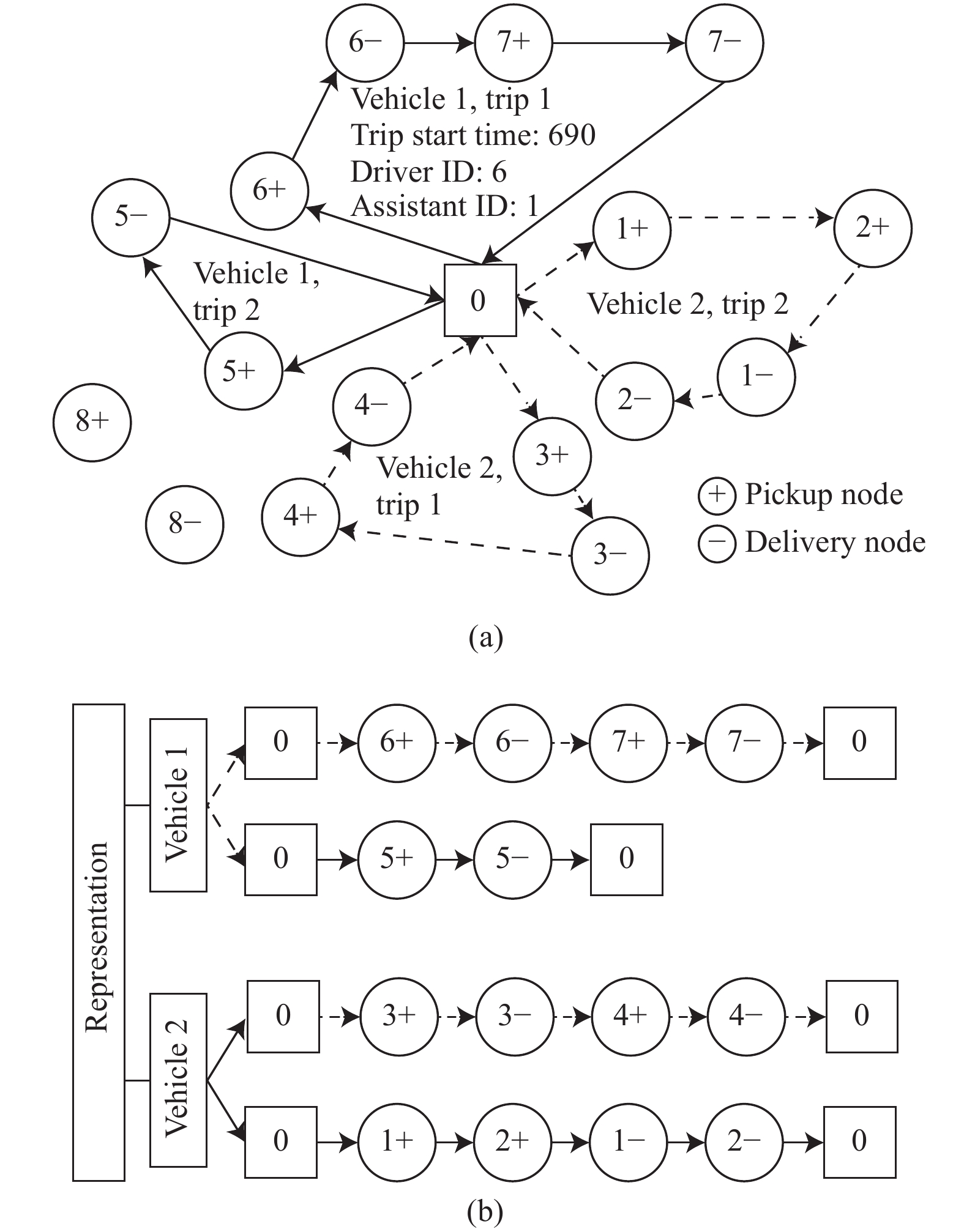
MTPDPTW-MP is formulated as a multiobjective problem (MO-MTPDPTWMP), which enables us to achieve a set of diverse and competitive solutions by addressing different objectives in a multiobjective manner. MO-MTPDPTWMP is a routing problem derived from the application of Hong Kong public hospitals, China. In this problem, the hospital can be regarded as the depot and ambulances can be regarded as vehicles. Each vehicle starts from the depot to accomplish some requests and returns to the depot within the maximum traveling duration. The goal of the problem is to design and schedule a set of optimal routes satisfying various constraints. Besides, the assignment of staff to vehicles should also be determined. A simple example with 8 requests and 2 vehicles is provided in Fig. 2 (a), in which there are 4 trips in total. The solution representation for this example is shown in Fig. 2 (b).
The inputs of the problem are as follows:
1) A complete undirected graph
2) The number of requests is
3) The node set
4) The edge set
5) Each node
6) Each edge
7) K denotes the set of available vehicles with heterogeneous capacity
8) M denotes the set of available staff. Each staff member
The output is a set of Pareto non-dominated solutions.
A feasible solution must satisfy the following constraints (
1) Pickup Before Delivery Constraint
2) Vehicle Capacity Constraint
3) Time Window Constraint
4) Maximum Duration Constraint
5) No Time Conflicting Constraint
6) Disinfection Time Constraint
7) Staff Demand Constraint
8) Staff Break Time Constraint
9) Staff Working Time Constraint
A solution of MO-MTPDPTWMP can be represented as a set of vehicle trips
| C=p∑i=0cvivi+1. | (1) |
Each trip has an assigned vehicle and it is a route that satisfies the following requirements: 1) Each trip starts and terminates at the depot and consists of a sequence of pickup and delivery nodes. 2) The start time is given for each trip. 3) Adequate staff are assigned to the trip. 4) There is no time conflict between any two trips of the same vehicle or assigned to the same staff member.
The following objectives reflect the conflicting interests of all stakeholders: the customers, hospital, and staff.
1) The Number of Unserved Requests
| f1=U | (2) |
where
2) Total Traveling Cost
| f2=|K|∑k=1uk∑j=1Ckj | (3) |
where
3) The Workload Deviation
| f3=|M|∑j=1|ωj−ˉω| | (4) |
where
More details about problem description and formulation can be found in [9].
ILS-VND was proposed in [9] to deal with MTPDPTW-MP, which is a single-objective optimization problem. A fixed weight vector for three objectives is used in the framework, where the number of unserved requests is set as the most important objective. As ILS-VND optimizes three objectives in a single-objective manner, only one final solution is returned to decision makers.
To the best of our knowledge, there is no publication dealing with the proposed MO-MTPDPTWMP. Solving it enables us to achieve a set of diverse and competitive solutions for decision makers by addressing different objectives in a multiobjective manner.
MOPs are problems with two or more objectives to be optimized simultaneously. An MOP with
| Minimize F(x)=(f1(x),f2(x),…,fm(x)), x∈Ω | (5) |
where
| PF={F(x)|x∈PS}. | (6) |
The goal of MOPs is to find a set of nondominated solutions with good performance in terms of both convergence and diversity. Convergence means that the solutions are close to the PF, while diversity means that the solutions are well distributed along the PF.
Metaheuristics are widely used algorithms for solving large and complex MOPs [15], [16]. Multiobjective metaheuristics algorithms can be roughly divided into two categories: multiobjective evolutionary algorithms (MOEAs) [15], including MOEA/D [17] and NSGA-II [18], and multiobjective local-search-based algorithms [16]. MOEAs simultaneously evolve a population of solutions. They show powerful exploration ability and can achieve high quality solutions for multiobjective continuous benchmark problems. Multiobjective local-search-based algorithms can promote search intensification and speed up convergence for multiobjective combinatorial optimization problems.
MOILS-ANS is a multiobjective local search algorithm. At every iteration of MOILS-ANS, a single solution is chosen and the local search is used to explore its neighbors. A novel adaptive neighborhood selection (ANS) strategy is designed and used in the local search process of MOILS-ANS. The ANS strategy adaptively selects neighborhood structures according to their past performances.
Algorithm 1 shows the main framework of MOILS-ANS. Two explicit sets of solutions (i.e., the current solution set
The main components of MOILS-ANS, including the initial solution construction, ANS strategy, perturbation, feasibility checking, and archive updating are described in detail as follows.
Algorithm 1 MOILS-ANS
Input: the current solution set’s size
Output: archive A
1 begin
2
3 initialize the current solution set
4 generate
5 while termination condition is not met do
6 randomly select a weight vector
7 the solution
8
9 while
10 perturb solution
11
12
13 if inserted then
14
15
16 else
17
18 end if
19 end while
20 update the current solution set
21 end while
22 return archive A;
23 end
The basic idea of generating an initial solution is to insert one request into the solution each time. RI heuristic [19] is used when selecting a request to insert. The method is useful for highly constrained problems and can construct high-quality initial solutions for further improvement. Relevant notations and formulas are as follows.
1)
2) If the request cannot be inserted into trip
3) For each request
4) The regret value of request
| RV=k∑i=1(ΔCh,xi−ΔCh,x1) | (7) |
where the parameter
The request with the maximum
Local search is one of general approaches with empirical success to combinatorial optimization problems. Its basic idea is that high-quality solutions can be found by iteratively improving a solution using modifications, called moves. A move type is specified by a neighborhood structure, which generates a neighborhood solution of the current solution [20]. The neighborhood solution of the current solution is evaluated after being generated. During the local search procedure, the weighted sum approach is often used to transform a multiobjective problem into a single-objective problem for evaluation as follows [2]:
| fws(x|λ)=m∑i=1λifi(x) | (8) |
where
1) Mutiple Neighborhood Structures: It is important to design multiple neighborhood structures in the local search when solving complex variants of the VRP [2], [6] or other combinatorial optimization problems [21], [22]. Using only one neighborhood structure may easily encounter the local optimum issue. Multiple neighborhood structures can broaden the exploration of the search space and help to escape the local optimum. In this paper, multiple neighborhood structures,
a)
b)
c)
d)
e)
f)
g)
In the neighborhood structures, all deletion/exchange operations are tried in a random order. Additionally, the
2) Adaptive Neighborhood Selection: How to flexibly coordinate multiple neighborhood structures to adapt to different instances of a problem or different stages of the search is a key challenge. In order to better combine multiple neighborhood structures, the concept of hyper-heuristics [24], [25] or adaptive operator selection [26] are adopted. Hence, this study proposes an adaptive neighborhood selection (ANS) strategy to tackle MO-MTPDPTWMP. Different from previous research [24]–[26], the proposed ANS is carefully designed for a multiobjective real-world combinatorial optimization problem rather than continuous benchmark problems or single-objective problems.
In each iteration of the local search, one neighborhood structure is selected to optimize the solution. The proposed ANS strategy adaptively selects neighborhood structures according to their previous performances, which is measured by the weighted-objective improvement
| z=fws(x|λ)−fws(x′|λ)fws(x|λ) | (9) |
where
By considering the weighted-objective improvement, neighborhood structures can be selected more appropriately during the local search process in ANS. There are
a)Neighborhood structures:
b) The performance of neighborhood structures on improving the weighted-objective value of solutions:
c) Selection probabilities of neighborhood structures:
Given the above notations, the performance
a) Suppose that
| zi=(1−α)×zi+α×z | (10) |
where the adaptation rate
b) The better the performance of
| pi=pmin | (11) |
where the minimum selection probability
The ANS strategy is shown in Algorithm 2. The input of ANS is a solution
Algorithm 2
Input: a solution
Output:
1 begin
2 for
3 select a neighborhood operator
4
5 if
6 calculate the weighted-objective improvement {
7 update the performance {
8 for
9 update the selection probability
10 end for
11
12 end if
13 end for
14 return
15 end
Perturbation is generally used to escape local optimum in metaheuristics. Its idea is to change the solution
The feasibility of a temporal solution should be checked when a request is inserted. The feasibility checking procedure consists of three steps: single trip checking, multitrip scheduling, and staff assignment. We should first check whether the inserted request will cause a single trip violating the first four constraints (
1) Single Trip Checking: The method is adopted from the segments concatenation developed by [7]–[9]. A segment is a sequence of consecutive nodes. For each trip, relevant information for all segments should be computed and saved in a preprocessing phase. When inserting or removing a request, different segments can be directly concatenated. The feasibility of a trip can be evaluated in constant time by using the relevant information of each segment.
For two segments
| D\left(\sigma \oplus {\sigma}'\right) = D\left(\sigma\right)+D\left({\sigma}'\right)+c_{\sigma_{j}{\sigma}'_{i}}+\Delta_{WT} | (12) |
| C\left(\sigma \oplus {\sigma}' \right) = C\left( \sigma \right)+C\left({\sigma}'\right)+d_{\sigma_{j}{\sigma}'_{i}} | (13) |
| E\left(\sigma \oplus {\sigma}' \right ) = {\max}\{E\left( {\sigma}'\right)-\Delta, E\left( \sigma \right)\}-\Delta_{WT} | (14) |
| L\left(\sigma \oplus {\sigma}' \right ) = {\min}\{L\left( {\sigma}'\right)-\Delta, L\left( \sigma \right)\} | (15) |
| Q\left(\sigma \oplus {\sigma}' \right) = Q\left( \sigma \right)+Q\left({\sigma}'\right) | (16) |
| PQ\left(\sigma \oplus {\sigma}' \right) = {\max}\{PQ\left( \sigma \right), Q\left( \sigma \right)+PQ\left( {\sigma}' \right)\} | (17) |
| SF\left(\sigma \oplus {\sigma}'\right) = {\max}\{SF\left( \sigma \right), SF\left( {\sigma}' \right)\} | (18) |
where
The new segment
2) Multitrip Scheduling: After the first step, all the trips are legal. Each vehicle may contain several trips. Multitrip scheduling should be performed to obtain a legal scheduling order for each vehicle.
After inserting or removing requests, a new trip is generated. First, we should check whether its original vehicle can still perform multitrip scheduling. If not, dispatch the trip to other vehicles until a legal scheduling order is found.
For a specific vehicle
| \begin{split} E\left(r_{i}\right) = & {\max}\{E\left(r_{i-1}\right)+D\left(r_{i-1}\right)+\delta, E\left(r_{i}\right)\}, \\ & \quad\;\;\;\;i = 2, ..., u \end{split} | (19) |
where
| \begin{split} L\left(r_{i}\right) = {\min}\{&L\left(r_{i+1}\right)-D\left(r_{i}\right)-\delta, L\left(r_{i}\right)\}, \\& i = u-1, ..., 1. \end{split} | (20) |
3) Staff Assignment: After the second step, the staff assignment procedure should be invoked for all the vehicles. A greedy heuristic is used to perform staff assignment.
Each time we select an unsettled trip with the earliest start time and try to assign a driver and sufficient assistants to the trip.
The feasibility checking for MO-MTPDPTWMP is sophisticated. More details about the feasibility checking can be referred to [7]–[9].
To obtain a set of Pareto nondominated solutions with good performance in terms of convergence and diversity, an external archive A with maximum size
The complexity of the proposed MOILS-ANS mainly depends on the local search in ANS strategy as shown in Algorithm 2, which has the highest complexity. The local search consists of different neighborhood structures. Among them, the most complex one is the
MOILS-ANS was coded in C++. All the experiments were conducted on a machine with Intel(R) Xeon(R) Gold 5118 2.30GHz CPU, 64 GB RAM, and the Ubuntu 16.04.5 operating system.
In MOILS-ANS, the size of the current solution set
In ANS, the search depth
Benchmark instances collected from public hospitals in Hong Kong, China are provided by [9]. An instance is constructed using the requests in a day. A total of 59 instances from January (31 instances) to February (28 instances) of 2009 are used to evaluate MOILS-ANS for MO-MTPDPTWMP. The format of an instance is 2009MMDD, where MM and DD denote the month and day, respectively. For example, 20090101 indicates daily requests on January 1st. There are 38 non-holiday instances and 21 holiday instances. In general, non-holiday instances have narrow time windows and extensive requests, while holiday instances have wide time windows and a few requests. The number of requests in all instances varies from 28 to 205. Each instance input consists of the following information:
1) Requests Data: available seats, staff demand, time windows, and service time.
2) Vehicle Data: vehicle number and vehicle capacity.
3) Staff Data: work period and lunch break for each staff.
4) Cost Matrix: traveling cost between any two locations.
The termination criterion is set to the maximum runtime [9]. Larger instances with more requests require more computation time, and thus the maximum runtime for each instance is set according to the number of requests as follows: 1800 seconds for
1) Performance Indicators: The performance of a multiobjective algorithm is evaluated in terms of convergence and diversity of the nondominated solutions obtained. Hypervolume (HV) and inverted generational distance (IGD) are two widely used indicators for performance evaluation. Therefore, we also adopt them in this study.
a) HV: The volume of the space enclosed by the solution set and a reference point is calculated as the HV value. For a minimization task, the larger the HV value is, the closer the solution set is to the Pareto front. In this work, the HV value is calculated based on the objective values normalized into [0, 1]. The reference point is set to (1.2, 1.2, 1.2).
b) IGD:The distance of the elements in the approximate Pareto front towards those in the true Pareto front is estimated as the IGD value. A smaller IGD indicates a better approximate Pareto set.
The true Pareto front of each instance is unknown. For each instance, all nondominated solutions produced by all algorithms over 20 runs are collected to form an approximation of its true Pareto front.
Additionally, two indicators proposed by [13] are used to compare nondominated solutions obtained by multiobjective algorithms with the best solution reported by the previous single-objective algorithm for MTPDPTW-MP [9]. Suppose that A is the set of all nondominated solutions in the objective space generated by a multiobjective algorithm and
a) Generated dominating solutions (GDS): GDS is the number of solutions in A that can dominate
| {\rm {GDS}}(A,s) = |\{a \in A|a\; {\rm{ dominates}}\; s\}|. | (21) |
b) Generated alternative solutions (GAS): GAS is the number of solutions in A that can be used as alternatives to
| {\rm GAS}(A,s) = |\{a \in A|\sum\limits_{i = 1}^{m}\frac{a_i-s_i-z_i^*}{z_i^{\rm nad}-z_i^{*}}<0\}| | (22) |
where
According to the above definitions, larger GDS and GAS indicate better nondominated solution sets.
2) Statistics by Wilcoxon and Friedman Tests: To test the significant differences between the results obtained by MOILS-ANS and other competitors on a single instance over 20 runs, single-problem Wilcoxon rank-sum test [29]–[31] at 5% significance level was carried out for each instance. Statistical results on sets of instances are summarized as
MO-MTPDPTWMP is a newly introduced problem in the literature and there is no existing algorithm applied to it yet. No existing results can be directly used for comparisons. Two competitor algorithms (MOILS-R and MOEA/D-ANS) are adopted for MO-MTPDPTWMP. Their characteristics are as follows.
1) MOILS-R: Unlike MOILS-ANS, MOILS-R randomly selects a neighborhood structure. The selection probabilities of different neighborhood structures are set to the same value. That is, seven neighborhood structures are selected uniformly. It is natural to adopt uniform selection probabilities for different neighborhood structures without prior knowledge about the performance of them. Comparing MOILS-ANS with MOILS-R, we can analyze the effect of the ANS strategy.
2) MOEA/D-ANS: MOEA/D [17] is adapted to form a state-of-the-art competitor for MO-MTPDPTWMP. MOEA/D is a representative MOEA [15]. A multiobjective optimization problem is decomposed into a number of scalar optimization subproblems in MOEA/D. These subproblems are optimized simultaneously. The algorithm optimizes each subproblem only using information from its several neighboring subproblems. According to [15], [17], [32], MOEA/D seems to be more suitable for tackling multiobjective combinatorial optimization problems than NSGA-II [18], because problem-specific (local search) techniques can be directly used to intensify the exploration of promising regions in the solution space. It provides a natural framework for using single-objective local search techniques [4]. ANS is embedded into MOEA/D to form a competitor called MOEA/D-ANS (shown in Algorithm 3).
For fair comparisons, the same algorithm components (initial solution construction, the ANS strategy, feasibility checking, and archive) described in Section III are also used in MOEA/D-ANS. The termination criterion of MOEA/D-ANS is also set to the maximum runtime as that in MOILS-ANS (Section IV-B). The number of weight vectors is set to
Algorithm 3 MOEA/D-ANS
Input: the number of weight vectors
Output: archive A
1 begin
2 A =
3 initialize population
4 generate
5 compute the neighborhood set B(i) =
6 while termination condition is not met do
7 for i = 1:
8 randomly select an index I from B(i);
9 x′ =
10 for each
11 if
12 xj = x′
13 end if
14 end for
15 updateArchive (A; x′);
16 end for
17 end while
18 return archive A;
19 end
Numerical values of performance indicators (HV and IGD) over 20 independent runs are shown in Table S1 in Appendix due to the limited space. Statistics summarizing those numerical values are shown in Tables I–IV. Table S1 in Appendix shows the HV and IGD values (mean and standard deviation (STD)) on all 59 instances. In terms of HV and IGD, the proposed MOILS-ANS obtains best mean values on 49 and 54 instances, respectively. In comparison, MOILS-R obtains best mean values on 4 and 3 instances. MOEA/D-ANS obtains best mean values on 6 and 2 instances, respectively. The results suggest that MOILS-ANS significantly outperforms MOILS-R and MOEA/D-ANS.
| {\rm {HV}} | w/t/l | R + | R − | p -value | \alpha = 0.05 | \alpha = 0.10 |
| MOILS-ANS vs MOILS-R | 47/11/1 | 1745.0 | 25.0 | 3.1364E–015 | YES | YES |
| \rm IGD | w/t/l | R + | R − | p -value | \alpha = 0.05 | \alpha = 0.10 |
| MOILS-ANS vs MOILS-R | 55/1/3 | 1744.0 | 26.0 | 3.7100E–015 | YES | YES |
 DownLoad:
CSV
DownLoad:
CSV
| HV | z -values | Unadjusted p -values | Adjusted p -values |
| MOILS-R vs MOILS-ANS | 6.996367 | 0.000000 | 0.016667 |
| MOILS-ANS vs MOEA/D-ANS | 6.259907 | 0.000000 | 0.025000 |
| MOILS-R vs MOEA/D-ANS | 0.736460 | 0.461451 | 0.050000 |
| IGD | z -values | Unadjusted p -values | Adjusted p -values |
| MOILS-R vs MOILS-ANS | 8.101057 | 0.000000 | 0.016667 |
| MOILS-ANS vs MOEA/D-ANS | 6.536080 | 0.000000 | 0.025000 |
| MOILS-R vs MOEA/D-ANS | 1.564977 | 0.117588 | 0.050000 |
DownLoad:
CSV
| Instances | HV | IGD | ||||
| MOILS-ANS | MOILS-R | MOEA/D-ANS | MOILS-ANS | MOILS-R | MOEA/D-ANS | |
| 20090101 | 0.7890 (0.0047) | 0.7850 (0.0042)– | 0.7669 (0.0192)– | 0.0552 (0.0042) | 0.0613 (0.0035)– | 0.0781 (0.0170)– |
| 20090102 | 0.6810 (0.0185) | 0.6417 (0.0224)– | 0.6178 (0.0346)– | 0.1068 (0.0102) | 0.1512 (0.0131)– | 0.1538 (0.0220)– |
| 20090103 | 0.7937 (0.0101) | 0.7842 (0.0133)– | 0.7739 (0.0237)– | 0.0689 (0.0072) | 0.0768 (0.0084)– | 0.0898 (0.0125)– |
| 20090104 | 0.7398 (0.0042) | 0.7366 (0.0076)= | 0.7145 (0.0118)– | 0.0535 (0.0025) | 0.0585 (0.0057)– | 0.0705 (0.0097)– |
| 20090105 | 0.6747 (0.0176) | 0.6025 (0.0643)– | 0.6232 (0.0254)– | 0.1123 (0.0194) | 0.1930 (0.0515)– | 0.1465 (0.0156)– |
| 20090106 | 0.6488 (0.0322) | 0.5754 (0.0684)– | 0.6021 (0.0254)– | 0.1483 (0.0233) | 0.2087 (0.0459)– | 0.1590 (0.0220)= |
| 20090107 | 0.6171 (0.0388) | 0.5794 (0.0559)– | 0.5937 (0.0337)– | 0.1451 (0.0251) | 0.2018 (0.0394)– | 0.1604 (0.0215)– |
| 20090108 | 0.5478 (0.0231) | 0.5015 (0.0530)– | 0.5734 (0.0259)+ | 0.1369 (0.0155) | 0.2032 (0.0430)– | 0.1419 (0.0074)= |
| 20090109 | 0.6278 (0.0248) | 0.5848 (0.0641)– | 0.6026 (0.0349)– | 0.1311 (0.0200) | 0.1774 (0.0399)– | 0.1521 (0.0144)– |
| 20090110 | 0.6354 (0.0115) | 0.6139 (0.0114)– | 0.6159 (0.0186)– | 0.0726 (0.0048) | 0.0890 (0.0079)– | 0.0948 (0.0108)– |
| 20090111 | 0.6989 (0.0063) | 0.6919 (0.0057)– | 0.6769 (0.0146)– | 0.0554 (0.0025) | 0.0602 (0.0038)– | 0.0742 (0.0094)– |
| 20090112 | 0.6622 (0.0214) | 0.6260 (0.0381)– | 0.6385 (0.0275)– | 0.1136 (0.0133) | 0.1630 (0.0335)– | 0.1300 (0.0174)– |
| 20090113 | 0.4561 (0.0895) | 0.3998 (0.0890)– | 0.4962 (0.0362)= | 0.2175 (0.0720) | 0.2706 (0.0594)– | 0.1583 (0.0173)+ |
| 20090114 | 0.6223 (0.0337) | 0.6023 (0.0638)= | 0.6413 (0.0344)= | 0.1329 (0.0199) | 0.1617 (0.0404)– | 0.1383 (0.0164)= |
| 20090115 | 0.6257 (0.0200) | 0.5948 (0.0532)– | 0.6074 (0.0307)– | 0.1333 (0.0215) | 0.1752 (0.0360)– | 0.1503 (0.0144)– |
| 20090116 | 0.6248 (0.0227) | 0.5664 (0.0685)– | 0.5844 (0.0187)– | 0.1358 (0.0155) | 0.1956 (0.0465)– | 0.1470 (0.0118)– |
| 20090117 | 0.6126 (0.0109) | 0.6044 (0.0109)= | 0.5990 (0.0187)– | 0.0650 (0.0030) | 0.0767 (0.0089)– | 0.0825 (0.0084)– |
| 20090118 | 0.6787 (0.0091) | 0.6816 (0.0051)= | 0.6552 (0.0129)– | 0.0639 (0.0102) | 0.0581 (0.0053)+ | 0.0810 (0.0100)– |
| 20090119 | 0.6093 (0.0182) | 0.5637 (0.0519)– | 0.6291 (0.0400)+ | 0.1178 (0.0148) | 0.1715 (0.0317)– | 0.1230 (0.0141)= |
| 20090120 | 0.6157 (0.0245) | 0.5779 (0.0684)= | 0.6024 (0.0243)= | 0.1428 (0.0209) | 0.1822 (0.0459)– | 0.1511 (0.0126)= |
| 20090121 | 0.6223 (0.0261) | 0.5561 (0.0805)– | 0.5748 (0.0258)– | 0.1428 (0.0211) | 0.1986 (0.0530)– | 0.1681 (0.0185)– |
| 20090122 | 0.5844 (0.0228) | 0.5349 (0.0486)– | 0.5618 (0.0353)– | 0.1405 (0.0176) | 0.1961 (0.0304)– | 0.1512 (0.0139)– |
| 20090123 | 0.6055 (0.0339) | 0.5494 (0.0471)– | 0.5685 (0.0259)– | 0.1578 (0.0270) | 0.2184 (0.0323)– | 0.1694 (0.0201)= |
| 20090124 | 0.5626 (0.0299) | 0.5502 (0.0223)= | 0.5361 (0.0271)– | 0.0682 (0.0076) | 0.0821 (0.0089)– | 0.0888 (0.0069)– |
| 20090125 | 0.7298 (0.0076) | 0.6998 (0.0100)– | 0.7158 (0.0173)– | 0.0605 (0.0025) | 0.0732 (0.0053)– | 0.0704 (0.0047)– |
| 20090126 | 0.7474 (0.0038) | 0.7335 (0.0033)– | 0.7353 (0.0160)– | 0.0480 (0.0023) | 0.0505 (0.0021)– | 0.0543 (0.0091)– |
| 20090127 | 0.7211 (0.0036) | 0.7216 (0.0030)= | 0.7137 (0.0080)– | 0.0559 (0.0022) | 0.0545 (0.0018)+ | 0.0627 (0.0039)– |
| 20090128 | 0.7298 (0.0088) | 0.7443 (0.0078)+ | 0.7461 (0.0041)+ | 0.0661 (0.0084) | 0.0493 (0.0058)+ | 0.0519 (0.0036)+ |
| 20090129 | 0.6394 (0.0179) | 0.6195 (0.0283)– | 0.6046 (0.0251)– | 0.1052 (0.0125) | 0.1336 (0.0188)– | 0.1324 (0.0132)– |
| 20090130 | 0.6351 (0.0189) | 0.6034 (0.0439)– | 0.5744 (0.0305)– | 0.1048 (0.0149) | 0.1466 (0.0268)– | 0.1394 (0.0183)– |
| 20090131 | 0.7152 (0.0109) | 0.6880 (0.0212)– | 0.6868 (0.0138)– | 0.0834 (0.0098) | 0.1169 (0.0159)– | 0.1148 (0.0111)– |
| 20090201 | 0.7145 (0.0046) | 0.6959 (0.0125)– | 0.6734 (0.0223)– | 0.0595 (0.0029) | 0.0751 (0.0080)– | 0.0928 (0.0188)– |
| 20090202 | 0.6760 (0.0239) | 0.6118 (0.0647)– | 0.6262 (0.0242)– | 0.1197 (0.0182) | 0.1727 (0.0412)– | 0.1454 (0.0162)– |
| 20090203 | 0.6128 (0.0295) | 0.5195 (0.0787)– | 0.5618 (0.0265)– | 0.1664 (0.0327) | 0.2422 (0.0428)– | 0.1789 (0.0197)= |
| 20090204 | 0.6260 (0.0453) | 0.5848 (0.0820)– | 0.5947 (0.0305)– | 0.1622 (0.0323) | 0.2139 (0.0504)– | 0.1757 (0.0196)– |
| 20090205 | 0.5787 (0.0269) | 0.5248 (0.0787)– | 0.5598 (0.0381)= | 0.1554 (0.0259) | 0.2181 (0.0491)– | 0.1531 (0.0190)= |
| 20090206 | 0.6349 (0.0164) | 0.6120 (0.0508)= | 0.6041 (0.0260)– | 0.1065 (0.0134) | 0.1373 (0.0333)– | 0.1312 (0.0127)– |
| 20090207 | 0.7130 (0.0067) | 0.6903 (0.0129)– | 0.6654 (0.0215)– | 0.0622 (0.0046) | 0.0789 (0.0075)– | 0.1003 (0.0090)– |
| 20090208 | 0.6639 (0.0098) | 0.6462 (0.0114)– | 0.6354 (0.0166)– | 0.0548 (0.0066) | 0.0752 (0.0099)– | 0.0752 (0.0135)– |
| 20090209 | 0.6300 (0.0316) | 0.5790 (0.0688)– | 0.6394 (0.0397)= | 0.1434 (0.0240) | 0.1974 (0.0446)– | 0.1500 (0.0163)= |
| 20090210 | 0.6264 (0.0219) | 0.5724 (0.0624)– | 0.5907 (0.0261)– | 0.1472 (0.0189) | 0.2035 (0.0386)– | 0.1660 (0.0172)– |
| 20090211 | 0.6671 (0.0171) | 0.6109 (0.0539)– | 0.6329 (0.0389)– | 0.1180 (0.0142) | 0.1790 (0.0303)– | 0.1496 (0.0164)– |
| 20090212 | 0.6113 (0.0246) | 0.5721 (0.0530)– | 0.5746 (0.0526)– | 0.1353 (0.0213) | 0.1834 (0.0332)– | 0.1667 (0.0206)– |
| 20090213 | 0.6699 (0.0303) | 0.6176 (0.0686)– | 0.5868 (0.0295)– | 0.1274 (0.0207) | 0.1820 (0.0408)– | 0.1827 (0.0199)– |
| 20090214 | 0.7489 (0.0058) | 0.7394 (0.0090)– | 0.7062 (0.0161)– | 0.0633 (0.0045) | 0.0703 (0.0080)– | 0.0944 (0.0078)– |
| 20090215 | 0.6966 (0.0066) | 0.6794 (0.0055)– | 0.6768 (0.0150)– | 0.0550 (0.0053) | 0.0599 (0.0054)– | 0.0647 (0.0066)– |
| 20090216 | 0.6511 (0.0135) | 0.6089 (0.0293)– | 0.6192 (0.0306)– | 0.1066 (0.0150) | 0.1490 (0.0195)– | 0.1255 (0.0147)– |
| 20090217 | 0.5600 (0.0328) | 0.5358 (0.0770)= | 0.5278 (0.0517)– | 0.1452 (0.0301) | 0.1891 (0.0475)– | 0.1642 (0.0290)– |
| 20090218 | 0.6281 (0.0192) | 0.6000 (0.0252)– | 0.5856 (0.0275)– | 0.1215 (0.0200) | 0.1649 (0.0227)– | 0.1367 (0.0148)– |
| 20090219 | 0.6444 (0.0394) | 0.5960 (0.0772)– | 0.6232 (0.0287)– | 0.1490 (0.0297) | 0.1974 (0.0457)– | 0.1556 (0.0136)= |
| 20090220 | 0.5946 (0.0345) | 0.5569 (0.0423)– | 0.5759 (0.0374)= | 0.1569 (0.0235) | 0.2103 (0.0408)– | 0.1628 (0.0145)= |
| 20090221 | 0.7512 (0.0056) | 0.7519 (0.0111)= | 0.7220 (0.0131)– | 0.0729 (0.0064) | 0.0807 (0.0141)= | 0.1065 (0.0152)– |
| 20090222 | 0.6143 (0.0063) | 0.6016 (0.0100)– | 0.5783 (0.0323)– | 0.0571 (0.0044) | 0.0682 (0.0060)– | 0.0855 (0.0227)– |
| 20090223 | 0.7076 (0.0133) | 0.7097 (0.0189)= | 0.6735 (0.0246)– | 0.0879 (0.0060) | 0.1080 (0.0133)– | 0.1197 (0.0091)– |
| 20090224 | 0.5466 (0.0307) | 0.5090 (0.0528)– | 0.5443 (0.0378)= | 0.1344 (0.0204) | 0.1926 (0.0455)– | 0.1467 (0.0118)– |
| 20090225 | 0.6963 (0.0254) | 0.6638 (0.0565)– | 0.6459 (0.0188)– | 0.0948 (0.0093) | 0.1414 (0.0394)– | 0.1342 (0.0136)– |
| 20090226 | 0.5967 (0.0267) | 0.5152 (0.0685)– | 0.5397 (0.0245)– | 0.1592 (0.0184) | 0.2348 (0.0554)– | 0.1934 (0.0176)– |
| 20090227 | 0.6213 (0.0303) | 0.5736 (0.0695)– | 0.6092 (0.0278)= | 0.1396 (0.0336) | 0.1809 (0.0422)– | 0.1509 (0.0148)– |
| 20090228 | 0.7646 (0.0050) | 0.7523 (0.0105)– | 0.7296 (0.0127)– | 0.0654 (0.0041) | 0.0806 (0.0094)– | 0.0961 (0.0124)– |
| w/t/l | 47/11/1 | 48/8/3 | 55/1/3 | 46/11/2 | ||
| “+”, “=” and “–” indicate that the result obtained by the corresponding competitor is significantly better than, similar to, and worse than the result obtained by MOILS-ANS, respectively. The best mean values of each instance are highlighted in bold. | ||||||
DownLoad:
CSV
1) Comparisons Between MOILS-ANS and MOILS-R: Table I provides the statistics of performance comparisons of MOILS-ANS and MOILS-R on 59 instances. Results in column
Moreover, the obtained
To visually demonstrate the performance of MOILS-ANS and its two competitor algorithms, the projections of nondominated solutions of MOILS-ANS, MOILS-R, and MOEA/D-ANS (in red, blue, and purple, respectively) on a selected instance 20090125 at
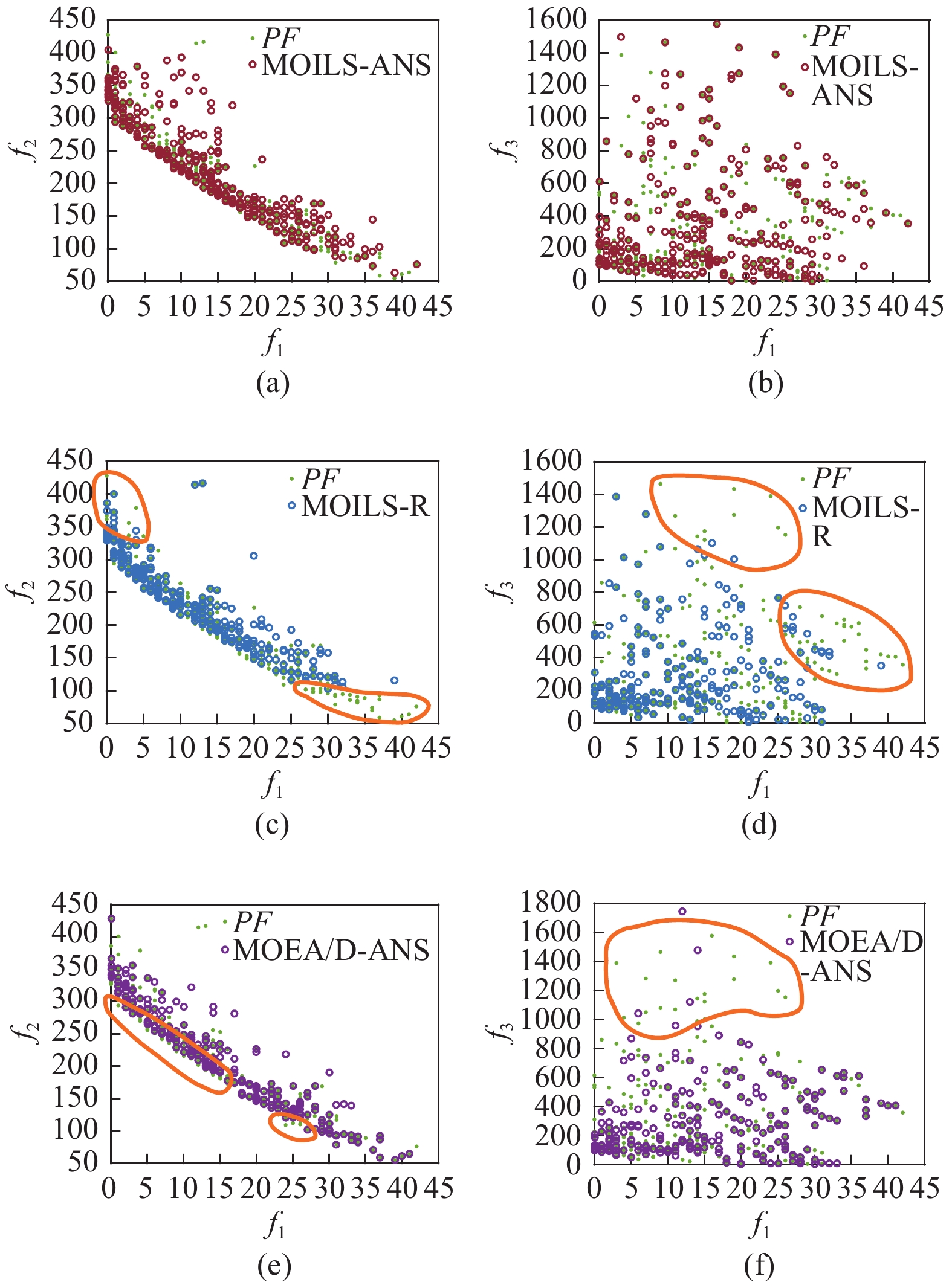
Comparing MOILS-ANS with MOILS-R from Fig. 3, we can easily find that some regions of the Pareto front are not fully covered or approximated by MOILS-R. As shown in Fig. 3(a), the final solution set obtained by MOILS-ANS spreads along the whole Pareto front, and is wider than those obtained by MOILS-R, as shown in Fig. 3(c). Comparing Figs. 3(b) and 3(d), we can find that MOILS-ANS covers all the regions of the Pareto front well, while MOILS-R misses some regions. Therefore, MOILS-ANS obtains better HV and IGD values than MOILS-R.
To sum up, MOILS-ANS outperforms MOILS-R. The effectiveness of the ANS strategy is revealed from comparisons between MOILS-ANS and MOILS-R.
2) Comparisons Between MOILS-ANS and MOEA/D-ANS: As summarized in Table II, MOILS-ANS significantly outperforms MOEA/D-ANS on 48 and 46 instances in terms of HV and IGD, respectively. Results of the multiproblem Wilcoxon signed-rank test show that MOILS-ANS is significantly better than MOEA/D-ANS in terms of HV and IGD.
| {\rm {HV}} | w/t/l | R + | R − | p -value | \alpha = 0.05 | \alpha = 0.10 |
| MOILS-ANS vs MOEA/D-ANS | 48/8/3 | 1659.0 | 111.0 | 4.5952E–011 | YES | YES |
| \rm IGD | w/t/l | R + | R − | p -value | \alpha = 0.05 | \alpha = 0.10 |
| MOILS-ANS vs MOEA/D-ANS | 46/11/2 | 1689.0 | 81.0 | 3.1537E–012 | YES | YES |
DownLoad:
CSV
Comparing MOILS-ANS with MOEA/D-ANS from Fig. 3, we can easily find that some regions of the Pareto front are not fully covered or approximated by MOEA/D-ANS. As shown in Fig. 3(e), although the final solution set obtained by MOEA/D-ANS spreads along the whole Pareto front, the solution set is not denser and closer to the true Pareto front as that of MOILS-ANS, as shown in Fig. 3(a). Moreover, comparisons between Figs. 3(b) and 3(f) show that MOEA/D-ANS misses some regions of the Pareto front, marked with the orange circle in Fig. 3(f).
Both MOILS-ANS and MOEA/D-ANS maintain and update a solution set, and they all can be seen as global search algorithms [16]. In MOILS-ANS, a solution in the current solution set is randomly selected for exploration and updating in each iteration, while, in MOEA/D-ANS, the whole population is explored and updated from generation to generation. The main characteristic of MOILS-ANS is that it extends the single-objective ILS framework [9] with perturbation scheme for escaping local minima [16]. Experimental results above show that MOILS-ANS performs better than MOEA/D-ANS. This might be due to the following reasons. In MOEA/D-ANS, it is likely that a high-quality solution will gradually fill the large portion of the population with its variants/copies because the neighborhood is defined based on uniformly distributed weight vectors. This may lead to a loss of diversity of the population in MOEA/D-ANS. In contrast, the perturbation mechanism of MOILS-ANS can help MOILS-ANS to escape local minima, which leads to better convergence of the obtained solution set.
3) Summary: Table III shows the average ranking of all algorithms by Friedman test on all instances. Table IV shows the test statistics and adjusted
| HV | Average ranking value | Final rank |
| MOILS-ANS | 1.1864 | 1 |
| MOEA/D-ANS | 2.3390 | 2 |
| MOILS-R | 2.4746 | 3 |
| IGD | Average ranking value | Final rank |
| MOILS-ANS | 1.1017 | 1 |
| MOEA/D-ANS | 2.3051 | 2 |
| MOILS-R | 2.5932 | 3 |
DownLoad:
CSV
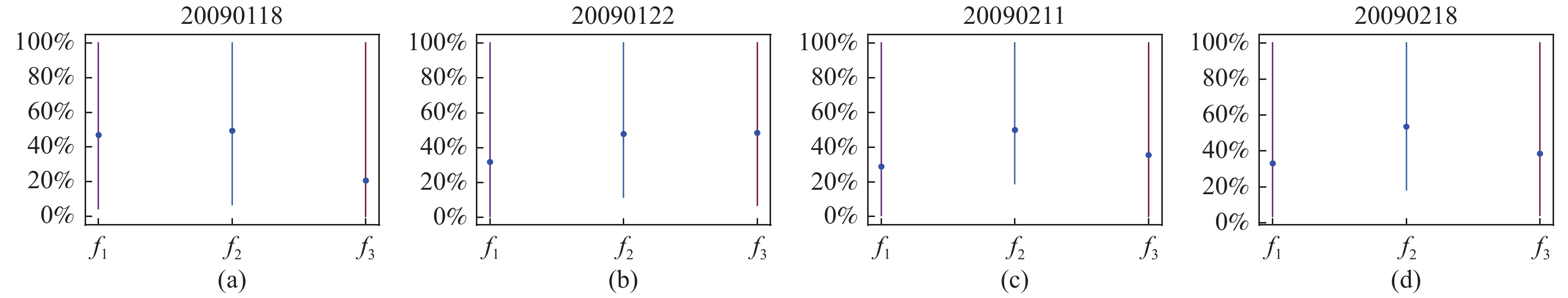
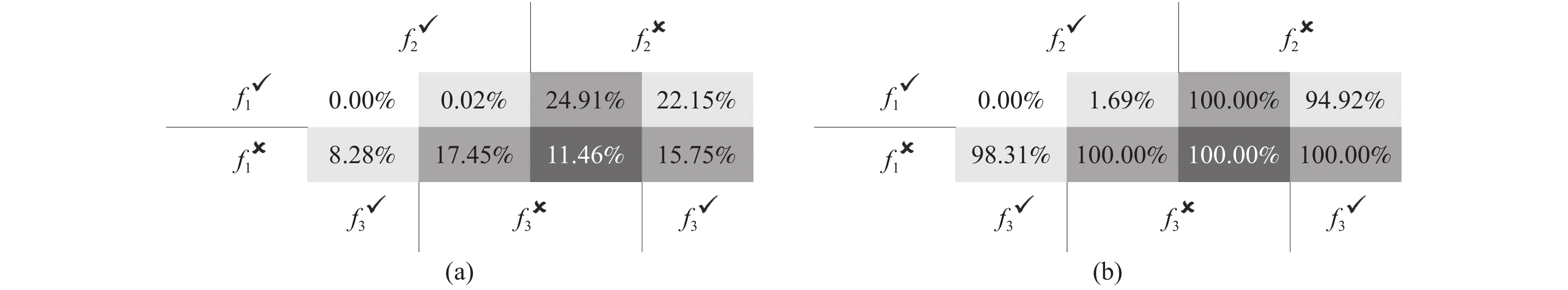
Understanding the nature of the relationships between objectives can help develop efficient and tailored problem-solving techniques in a multiobjective optimization problem. Usually, important properties of objectives and relationships between them can be revealed from the PF. Therefore, this study uses the method proposed recently in [33] to visualize and analyze the nature of objectives through the PF. For each instance, the approximate PFmentioned in Section IV-C is used as PF since the true PF is unknown. Four randomly selected instances (i.e., 20090118, 20090122, 20090211, and 20090218) from all instances of January and February are chosen as representatives for analysis. We follow the four analysis steps used in [33]. The corresponding analysis results are shown in Figs. S1–S5 in the Appendix. Observations can be concluded as follows.
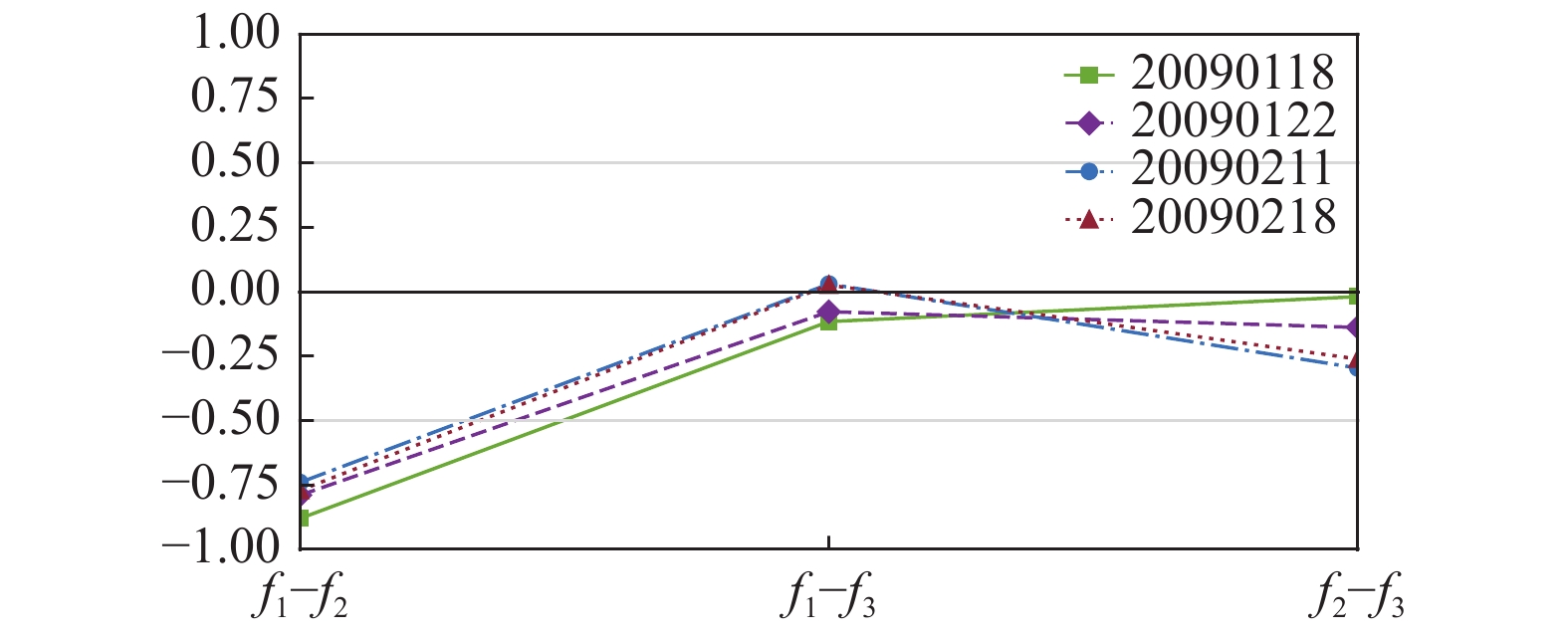

1) The pairwise correlation values in Fig. S1 and the scatter plots in Fig. S5 show that conflicting relationship exists between
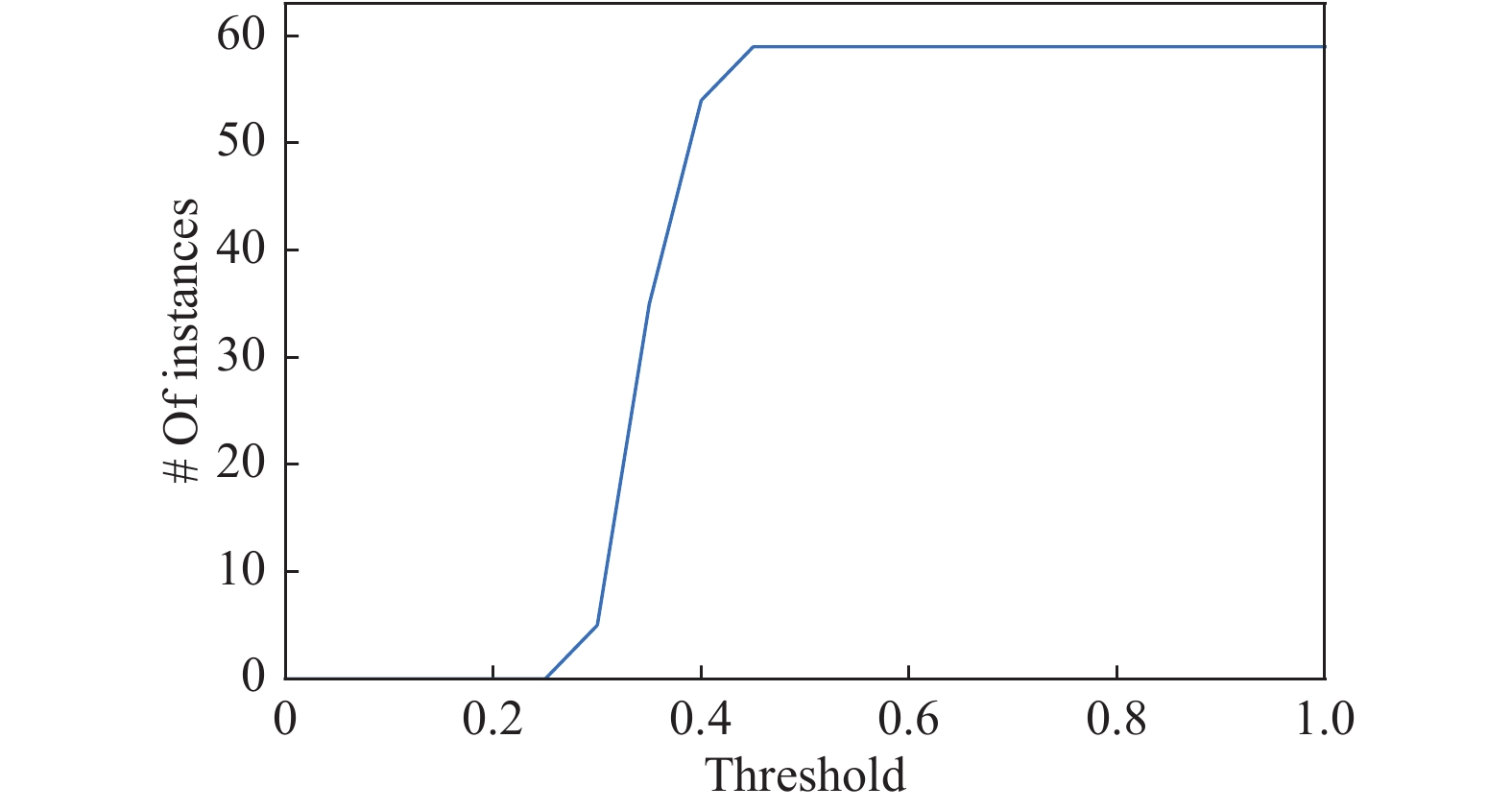
2) Fig. S4(a) shows that almost all regions have solutions, representing a wide variety of options for decision makers. Besides, Fig. S4(b) shows that the frequency of instances is high in most regions, meaning that the fitness landscapes of instances are alike. That is, recurring features exist in the fitness landscapes of different instances. Using this characteristic, it may be wise to solve one instance of a given problem scenario using computationally expensive multiobjective algorithms to obtain a good approximation set and then using goal programming with efficient single-objective algorithms to solve other instances of the same problem scenario [34].
1) Comparison Results: A single-objective algorithm called ILS-VND was proposed in [9] to deal with single-objective MTPDPTW-MP. The best solutions generated by ILS-VND are collected for comparisons since the same instances are solved by both multiobjective algorithms and ILS-VND. For each instance, all nondominated solutions generated by a multiobjective algorithm over 20 runs are combined to form its nondominated solution set, which is used to compare with the best solution generated by ILS-VND.
Table S2 in Appendix summarizes GDS and GAS values of MOILS-ANS, MOILS-R, and MOEA/D-ANS with respect to best solutions of ILS-VND for each instance. Table S3 in Appendix summarizes the number of nondominated solutions generated by MOILS-ANS, MOILS-R, and MOEA/D-ANS for each instance. Key observations can be found as follows.
| Instances | MOILS-ANS | MOILS-R | MOEA/D-ANS | |||
| GDS | GAS | GDS | GAS | GDS | GAS | |
| 20090101 | 0 | 196 | 0 | 228 | 0 | 200 |
| 20090102 | 0 | 307 | 0 | 301 | 0 | 248 |
| 20090103 | 0 | 267 | 0 | 290 | 0 | 242 |
| 20090104 | 0 | 192 | 0 | 162 | 0 | 193 |
| 20090105 | 0 | 370 | 0 | 278 | 0 | 278 |
| 20090106 | 0 | 324 | 0 | 206 | 0 | 189 |
| 20090107 | 0 | 356 | 0 | 251 | 0 | 306 |
| 20090108 | 0 | 363 | 0 | 305 | 0 | 219 |
| 20090109 | 0 | 347 | 0 | 298 | 0 | 250 |
| 20090110 | 0 | 209 | 0 | 233 | 0 | 215 |
| 20090111 | 0 | 233 | 0 | 255 | 0 | 233 |
| 20090112 | 0 | 313 | 0 | 334 | 0 | 278 |
| 20090113 | 0 | 359 | 0 | 282 | 0 | 373 |
| 20090114 | 0 | 248 | 0 | 276 | 0 | 229 |
| 20090115 | 0 | 385 | 0 | 396 | 0 | 284 |
| 20090116 | 0 | 357 | 0 | 293 | 0 | 346 |
| 20090117 | 0 | 277 | 0 | 270 | 0 | 242 |
| 20090118 | 0 | 213 | 0 | 213 | 0 | 202 |
| 20090119 | 0 | 323 | 0 | 324 | 0 | 307 |
| 20090120 | 0 | 216 | 0 | 215 | 0 | 202 |
| 20090121 | 0 | 321 | 0 | 290 | 0 | 235 |
| 20090122 | 0 | 276 | 0 | 231 | 0 | 176 |
| 20090123 | 0 | 408 | 0 | 332 | 0 | 276 |
| 20090124 | 0 | 266 | 0 | 264 | 0 | 257 |
| 20090125 | 0 | 164 | 0 | 193 | 0 | 116 |
| 20090126 | 0 | 173 | 0 | 205 | 0 | 155 |
| 20090127 | 0 | 199 | 0 | 261 | 0 | 184 |
| 20090128 | 0 | 121 | 0 | 170 | 0 | 104 |
| 20090129 | 0 | 295 | 0 | 350 | 0 | 251 |
| 20090130 | 0 | 334 | 0 | 319 | 0 | 271 |
| 20090131 | 0 | 252 | 0 | 330 | 0 | 169 |
| 20090201 | 0 | 199 | 0 | 170 | 0 | 201 |
| 20090202 | 0 | 220 | 0 | 198 | 0 | 120 |
| 20090203 | 0 | 308 | 0 | 176 | 0 | 222 |
| 20090204 | 0 | 363 | 0 | 279 | 0 | 274 |
| 20090205 | 0 | 379 | 0 | 260 | 0 | 267 |
| 20090206 | 0 | 327 | 0 | 323 | 0 | 257 |
| 20090207 | 0 | 307 | 0 | 333 | 0 | 206 |
| 20090208 | 0 | 227 | 0 | 217 | 0 | 219 |
| 20090209 | 0 | 311 | 0 | 246 | 0 | 247 |
| 20090210 | 0 | 323 | 0 | 351 | 0 | 267 |
| 20090211 | 0 | 372 | 0 | 336 | 0 | 289 |
| 20090212 | 0 | 374 | 0 | 364 | 0 | 272 |
| 20090213 | 0 | 314 | 0 | 312 | 0 | 224 |
| 20090214 | 0 | 159 | 0 | 185 | 0 | 142 |
| 20090215 | 0 | 125 | 0 | 214 | 0 | 135 |
| 20090216 | 0 | 385 | 0 | 435 | 0 | 305 |
| 20090217 | 0 | 428 | 0 | 369 | 0 | 326 |
| 20090218 | 0 | 358 | 0 | 312 | 0 | 266 |
| 20090219 | 0 | 374 | 0 | 307 | 0 | 282 |
| 20090220 | 0 | 436 | 0 | 312 | 0 | 288 |
| 20090221 | 0 | 247 | 0 | 255 | 0 | 214 |
| 20090222 | 0 | 147 | 0 | 154 | 0 | 169 |
| 20090223 | 0 | 295 | 0 | 325 | 0 | 272 |
| 20090224 | 0 | 452 | 0 | 378 | 0 | 356 |
| 20090225 | 0 | 334 | 0 | 365 | 0 | 249 |
| 20090226 | 0 | 409 | 0 | 352 | 0 | 272 |
| 20090227 | 0 | 365 | 0 | 281 | 0 | 295 |
| 20090228 | 0 | 266 | 0 | 271 | 0 | 235 |
| Average | 0 | 296.0678 | 0 | 278.5593 | 0 | 239.0000 |
| The best GAS values of each instance are highlighted in bold. | ||||||
DownLoad:
CSV
| Instances | No. of generated nondominated solutions | ||
| MOILS-ANS | MOILS-R | MOEA/D-ANS | |
| 20090101 | 226 | 243 | 218 |
| 20090102 | 341 | 306 | 267 |
| 20090103 | 316 | 305 | 262 |
| 20090104 | 254 | 250 | 250 |
| 20090105 | 373 | 313 | 299 |
| 20090106 | 366 | 234 | 299 |
| 20090107 | 381 | 261 | 379 |
| 20090108 | 426 | 325 | 301 |
| 20090109 | 384 | 363 | 298 |
| 20090110 | 221 | 238 | 217 |
| 20090111 | 256 | 288 | 286 |
| 20090112 | 349 | 346 | 285 |
| 20090113 | 359 | 282 | 373 |
| 20090114 | 370 | 346 | 310 |
| 20090115 | 387 | 396 | 285 |
| 20090116 | 392 | 324 | 359 |
| 20090117 | 295 | 287 | 268 |
| 20090118 | 262 | 245 | 233 |
| 20090119 | 323 | 324 | 307 |
| 20090120 | 404 | 312 | 285 |
| 20090121 | 333 | 321 | 260 |
| 20090122 | 362 | 312 | 332 |
| 20090123 | 418 | 332 | 277 |
| 20090124 | 316 | 273 | 286 |
| 20090125 | 276 | 235 | 220 |
| 20090126 | 239 | 247 | 230 |
| 20090127 | 296 | 313 | 249 |
| 20090128 | 186 | 240 | 223 |
| 20090129 | 330 | 350 | 256 |
| 20090130 | 363 | 328 | 277 |
| 20090131 | 363 | 381 | 241 |
| 20090201 | 274 | 260 | 238 |
| 20090202 | 372 | 347 | 308 |
| 20090203 | 346 | 217 | 294 |
| 20090204 | 372 | 303 | 290 |
| 20090205 | 381 | 277 | 273 |
| 20090206 | 396 | 371 | 300 |
| 20090207 | 331 | 356 | 228 |
| 20090208 | 252 | 225 | 239 |
| 20090209 | 404 | 355 | 310 |
| 20090210 | 364 | 369 | 277 |
| 20090211 | 387 | 341 | 295 |
| 20090212 | 377 | 371 | 277 |
| 20090213 | 378 | 355 | 270 |
| 20090214 | 330 | 324 | 254 |
| 20090215 | 304 | 274 | 267 |
| 20090216 | 385 | 435 | 306 |
| 20090217 | 428 | 369 | 328 |
| 20090218 | 358 | 313 | 267 |
| 20090219 | 395 | 319 | 299 |
| 20090220 | 436 | 312 | 290 |
| 20090221 | 306 | 297 | 270 |
| 20090222 | 147 | 154 | 170 |
| 20090223 | 295 | 328 | 272 |
| 20090224 | 453 | 378 | 356 |
| 20090225 | 345 | 386 | 265 |
| 20090226 | 409 | 366 | 283 |
| 20090227 | 380 | 332 | 337 |
| 20090228 | 314 | 318 | 300 |
| Average | 340.4407 | 311.3898 | 279.5763 |
| The largest number of nondominated solutions of each instance are highlighted in bold. | |||
DownLoad:
CSV
a) All GDS values are zero. The single-objective algorithm invests all computing resources to optimize three objectives with a fixed weight vector, and returns just one solution finally. In contrast, the proposed multiobjective algorithm must make a balance among three objectives and return a set of tradeoff solutions finally. Therefore, it is quite difficult for the proposed algorithm to dominate the solution generated by the single-objective algorithm for MO-MTPDPTWMP. In this regard, all GDS values are 0. It suggests that the proposed algorithm may still have room for further improvement in future.
b) For each instance, GAS values show that each algorithm can generate numerous alternative solutions with respect to the best solution. These alternative solutions can provide decision makers with a wide variety of options to best suit their specific requirements [13], [14].
c) The proposed MOILS-ANS obtains the best GAS values on most instances (32 instances, about 54.24% of all 59 instances). Besides, the average GAS value of MOILS-ANS is the best among all multiobjective algorithms.
To sum up, MOILS-ANS performs best, which is in line with our previous analysis based on HV and IGD.
2) Benefits of Multiobjective Optimization: To illustrate the benefits of multiobjective MTPDPTW-MP, alternative solutions generated by MOILS-ANS on four selected instances (i.e., 20090118, 20090122, 20090211, and 20090218) are visualized using parallel coordinates in Fig. 4. Our three objective functions are represented as three vertical axes in parallel coordinates. Each solution (a 3-D vector) is drawn as a polyline with vertices on the parallel axes, and the position of the vertex on the
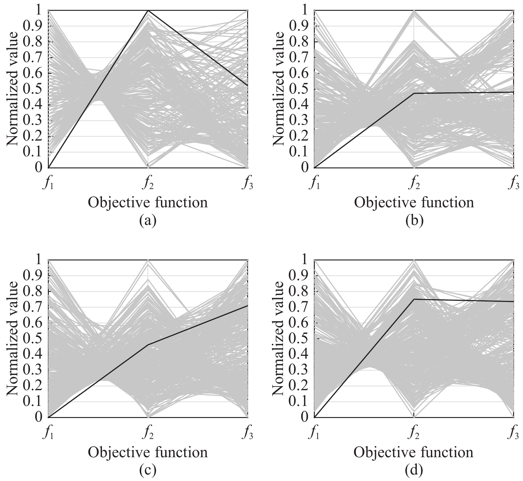
a) For each instance, MOILS-ANS generates numerous alternatives with respect to the best solution. These alternatives can help decision makers to better understand the situation of the problem and provide them with more flexibility to select a solution that best matches their requirements. If all objectives are simply combined into a single one like ILS-VND, many alternatives will be lost during the search process.
b) Best solutions reported by ILS-VND always have good performances on
c) Because of the inter-dependency among different objectives, a solution with the best performance on one objective has to compromise some other objectives. Therefore, “extreme” solutions with the best value for one objective may not be acceptable to decision makers. For example, customer-oriented solutions (black lines in Fig. 4) provided by ILS-VND are the best in terms of
This study formulates MTPDPTW-MP as a multiobjective optimization problem to better meet the requirements of different stakeholders in real-world scenarios. To solve MO-MTPDPTWMP, a multiobjective algorithm MOILS-ANS is proposed. Problem-specific neighborhood structures and an adaptive neighborhood selection strategy are designed to better explore the search space. Experimental results show that MOILS-ANS is significantly better than the other two multiobjective algorithms. The nondominated solutions obtained by all multiobjective algorithms for MO-MTPDPTWMP are mined. The nature of objective functions and important properties of the problem are revealed. Moreover, by comparing solutions generated by MOILS-ANS with the best solutions generated by the previous single-objective algorithm, the benefits of multiobjective optimization are summarized. The mining and analysis make a step toward explainable multiobjective optimization.
In the future, this study can be extended from several aspects. Firstly, the proposed algorithm requires a great deal of time when dealing with large scale instances. Therefore, the proposed algorithm can be speeded up through modern computing architectures, such as computer cluster and GPU, as in [35]. It also can be extended to solve other multiobjective routing and scheduling problems [1]. Secondly, the crossover operator is not adopted in the proposed algorithm and MOEA/D-ANS is in consistent with the existing multiobjective algorithms [2], [36]–[41]. Previous experience [38] showed that the crossover of solutions in a highly constrained problem always produces infeasible solutions. Feasibility checking is too sophisticated for MO-MTPDPTWMP. This means that a good crossover operator or repairing heuristics need to be designed, and thus the application of crossover-based algorithms to MO-MTPDPTWMP is a possible research direction. Finally, the properties of MO-MTPDPTWMP can be further studied from nondominated solutions generated by the proposed algorithms. Making full use of problem-specific knowledge can improve the search ability of multiobjective algorithms. Selection of proper hyperparameters of the algorithms using the method in [42], [43] is also our future work.

| [1] |
L. Wang and J. Lu, “A memetic algorithm with competition for the capacitated green vehicle routing problem,” IEEE/CAA J. Autom. Sinica, vol. 6, no. 2, pp. 516–526, 2019. doi: 10.1109/JAS.2019.1911405
|
| [2] |
J. Wang, L. Yuan, Z. Zhang, S. Gao, Y. Sun, and Y. Zhou, “Multiobjective multiple neighborhood search algorithms for multiobjective fleet size and mix location-routing problem with time windows,” IEEE Trans. Systems,Man,and Cybernetics:Systems, 2019. doi: 10.1109/TSMC.2019.2912194
|
| [3] |
J. Wang, T. Weng, and Q. Zhang, “A two-stage multiobjective evolutionary algorithm for multiobjective multi-depot vehicle routing problem with time windows,” IEEE Trans. Cybernetics, vol. 49, no. 7, pp. 2467–2478, 2019. doi: 10.1109/TCYB.2018.2821180
|
| [4] |
J. Wang, Y. Zhou, Y. Wang, J. Zhang, C. P. Chen, and Z. Zheng, “Multiobjective vehicle routing problems with simultaneous delivery and pickup and time windows: formulation, instances and algorithms,” IEEE Trans. Cybernetics, vol. 46, no. 3, pp. 582–594, 2016. doi: 10.1109/TCYB.2015.2409837
|
| [5] |
G. Kim, Y.-S. Ong, C. K. Heng, P. S. Tan, and N. A. Zhang, “City vehicle routing problem (city VRP): A review,” IEEE Trans. Intelligent Transportation Systems, vol. 16, no. 4, pp. 1654–1666, 2015. doi: 10.1109/TITS.2015.2395536
|
| [6] |
U. Derigs and M. Pullmann, “A computational study comparing different multiple neighbourhood strategies for solving rich vehicle routing problems,” IMA J. Management Mathematics, vol. 27, no. 1, pp. 3–23, 2016. doi: 10.1093/imaman/dpt022
|
| [7] |
T. Vidal, T. G. Crainic, M. Gendreau, and C. Prins, “A hybrid genetic algorithm with adaptive diversity management for a large class of vehicle routing problems with time-windows,” Computers&Operations Research, vol. 40, no. 1, pp. 475–489, 2013.
|
| [8] |
T. Vidal, T. G. Crainic, M. Gendreau, and C. Prins, “A unified solution framework for multi-attribute vehicle routing problems,” European J. Operational Research, vol. 234, no. 3, pp. 658–673, 2014. doi: 10.1016/j.ejor.2013.09.045
|
| [9] |
A. Lim, Z. Zhang, and H. Qin, “Pickup and delivery service with manpower planning in Hong Kong public hospitals,” Transportation Science, vol. 51, no. 2, pp. 688–705, 2016.
|
| [10] |
Z. Zhang, H. Qin, K. Wang, H. He, and T. Liu, “Manpower allocation and vehicle routing problem in non-emergency ambulance transfer service,” Transportation Research Part E, vol. 106, pp. 45–59, 2017. doi: 10.1016/j.tre.2017.08.002
|
| [11] |
Y. Cai, Z. Zhang, S. Guo, H. Qin, and A. Lim, “A tree-based tabu search for the manpower allocation problem with time windows and job-teaming constraints,” in Proc. 23rd Int. Joint Conf. Artificial Intelligence, 2013, pp. 496–502.
|
| [12] |
Y. Yu, S. Gao, Y. Wang, and Y. Todo, “Global optimum-based search differential evolution,” IEEE/CAA J. Autom. Sinica, vol. 6, no. 2, pp. 379–394, 2019. doi: 10.1109/JAS.2019.1911378
|
| [13] |
M. A. Nayeem, M. M. Islam, and X. Yao, “Solving transit network design problem using many-objective evolutionary approach,” IEEE Trans. Intelligent Transportation Systems, vol. 20, no. 10, pp. 3952–3963, 2019. doi: 10.1109/TITS.2018.2883511
|
| [14] |
A. Gupta, C. K. Heng, Y.-S. Ong, P. S. Tan, and A. N. Zhang, “A generic framework for multi-criteria decision support in eco-friendly urban logistics systems,” Expert Systems With Applications, vol. 71, pp. 288–300, 2017. doi: 10.1016/j.eswa.2016.09.033
|
| [15] |
A. Zhou, B.-Y. Qu, H. Li, S.-Z. Zhao, P. N. Suganthan, and Q. Zhang, “Multiobjective evolutionary algorithms: A survey of the state of the art,” Swarm and Evolutionary Computation, vol. 1, no. 1, pp. 32–49, 2011. doi: 10.1016/j.swevo.2011.03.001
|
| [16] |
A. Blot, M.-É. Kessaci, and L. Jourdan, “Survey and unification of local search techniques in metaheuristics for multi-objective combinatorial optimisation,” J. Heuristics, vol. 24, no. 6, pp. 853–877, 2018. doi: 10.1007/s10732-018-9381-1
|
| [17] |
Q. Zhang and H. Li, “MOEA/D: A multiobjective evolutionary algorithm based on decomposition,” IEEE Trans. Evolutionary Computation, vol. 11, no. 6, pp. 712–731, 2007. doi: 10.1109/TEVC.2007.892759
|
| [18] |
K. Deb, A. Pratap, S. Agarwal, and T. Meyarivan, “A fast and elitist multiobjective genetic algorithm: NSGA-II,” IEEE Trans. Evolutionary Computation, vol. 6, no. 2, pp. 182–197, 2002. doi: 10.1109/4235.996017
|
| [19] |
M. Diana and M. M. Dessouky, “A new regret insertion heuristic for solving large-scale dial-a-ride problems with time windows,” Transportation Research Part B:Methodological, vol. 38, no. 6, pp. 539–557, 2004. doi: 10.1016/j.trb.2003.07.001
|
| [20] |
F. Arnold and K. Sörensen, “Knowledge-guided local search for the vehicle routing problem,” Computers&Operations Research, vol. 105, pp. 32–46, 2019.
|
| [21] |
S. Abdullah and H. Turabieh, “On the use of multi neighbourhood structures within a tabu-based memetic approach to university timetabling problems,” Information Sciences, vol. 191, pp. 146–168, 2012. doi: 10.1016/j.ins.2011.12.018
|
| [22] |
H. Ishibuchi, Y. Hitotsuyanagi, N. Tsukamoto, and Y. Nojima, “Use of heuristic local search for single-objective optimization in multiobjective memetic algorithms,” in Proc. Int. Conf. Parallel Problem Solving from Nature. Springer, 2008, pp. 743–752.
|
| [23] |
O. Bräysy and M. Gendreau, “Vehicle routing problem with time windows, part I: Route construction and local search algorithms,” Transportation Science, vol. 39, no. 1, pp. 104–118, 2005. doi: 10.1287/trsc.1030.0056
|
| [24] |
E. K. Burke, M. Gendreau, M. Hyde, G. Kendall, G. Ochoa, E. Özcan, and R. Qu, “Hyper-heuristics: A survey of the state of the art,” J. Operational Research Society, vol. 64, no. 12, pp. 1695–1724, 2013. doi: 10.1057/jors.2013.71
|
| [25] |
N. Pillay and R. Qu, Hyper-Heuristics: Theory and Applications, Natural Computing Series. Springer, 2018.
|
| [26] |
N. Hitomi and D. Selva, “A classification and comparison of credit assignment strategies in multiobjective adaptive operator selection,” IEEE Trans. Evolutionary Computation, vol. 21, no. 2, pp. 294–314, 2017. doi: 10.1109/TEVC.2016.2602348
|
| [27] |
W. Hu and G. G. Yen, “Adaptive multiobjective particle swarm optimization based on parallel cell coordinate system,” IEEE Trans. Evolutionary Computation, vol. 19, no. 1, pp. 1–18, 2015. doi: 10.1109/TEVC.2013.2296151
|
| [28] |
I. Das and J. E. Dennis, “Normal-boundary intersection: A new method for generating the Pareto surface in nonlinear multicriteria optimization problems,” SIAM J. Optimization, vol. 8, no. 3, pp. 631–657, 1998. doi: 10.1137/S1052623496307510
|
| [29] |
F. Wilcoxon, “Individual comparisons by ranking methods,” Biometrics Bulletin, vol. 1, no. 6, pp. 80–83, 1945. doi: 10.2307/3001968
|
| [30] |
J. Derrac, S. García, D. Molina, and F. Herrera, “A practical tutorial on the use of nonparametric statistical tests as a methodology for comparing evolutionary and swarm intelligence algorithms,” Swarm and Evolutionary Computation, vol. 1, no. 1, pp. 3–18, 2011. doi: 10.1016/j.swevo.2011.02.002
|
| [31] |
J. Alcalá-Fdez, L. Sánchez, S. García, M. del Jesus, S. Ventura, J. Garrell, J. Otero, C. Romero, J. Bacardit, V. Rivas, J. Fernández, and F. Haerrera, “KEEL: A software tool to assess evolutionary algorithms for data mining problems,” Soft Computing, vol. 13, no. 3, pp. 307–318, 2009. doi: 10.1007/s00500-008-0323-y
|
| [32] |
Y. Mei, K. Tang, and X. Yao, “Decomposition-based memetic algorithm for multiobjective capacitated arc routing problem,” IEEE Trans. Evolutionary Computation, vol. 15, no. 2, pp. 151–165, 2011. doi: 10.1109/TEVC.2010.2051446
|
| [33] |
R. L. Pinheiro, D. Landa-Silva, and J. Atkin, “A technique based on trade-off maps to visualise and analyse relationships between objectives in optimisation problems,” J. Multi-Criteria Decision Analysis, vol. 24, no. 1-2, pp. 37–56, 2017. doi: 10.1002/mcda.1604
|
| [34] |
R. L. Pinheiro, D. Landa-Silva, W. Laesanklang, and A. A. Constantino, “An efficient application of goal programming to tackle multiobjective problems with recurring fitness landscapes,” in Proc. 7th Int. Conf. Operations Research and Enterprise Systems, 2018.
|
| [35] |
Z. Zhang, Y. Sun, H. Xie, Y. Teng, and J. Wang, “GMMA: GPU based multiobjective memetic algorithms for vehicle routing problem with route balancing,” Applied Intelligence, vol. 49, no. 1, pp. 63–78, 2019. doi: 10.1007/s10489-018-1210-6
|
| [36] |
Y. Xu and R. Qu, “Solving multi-objective multicast routing problems by evolutionary multi-objective simulated annealing algorithms with variable neighbourhoods,” J. Operational Research Society, vol. 62, no. 2, pp. 313–325, 2011. doi: 10.1057/jors.2010.138
|
| [37] |
H. Li and D. Landa-Silva, “An adaptive evolutionary multi-objective approach based on simulated annealing,” Evolutionary Computation, vol. 19, no. 4, pp. 561–595, 2011. doi: 10.1162/EVCO_a_00038
|
| [38] |
E. Burke and J. Landa Silva, “The influence of the fitness evaluation method on the performance of multiobjective search algorithms,” European J. Operational Research, vol. 169, no. 3, pp. 875–897, 2006. doi: 10.1016/j.ejor.2004.08.028
|
| [39] |
L. Ke, Q. Zhang, and R. Battiti, “Hybridization of decomposition and local search for multiobjective optimization,” IEEE Trans. Cybernetics, vol. 44, no. 10, pp. 1808–1820, 2014. doi: 10.1109/TCYB.2013.2295886
|
| [40] |
B. Derbel, A. Liefooghe, Q. Zhang, H. Aguirre, and K. Tanaka, “Multi-objective local search based on decomposition,” Lecture Notes in Computer Science, vol. 9921 LNCS, pp. 431–441, 2016. doi: 10.1007/978-3-319-45823-6_40
|
| [41] |
J. Shi, Q. Zhang, and J. Sun, “PPLS/D: Parallel Pareto local search based on decomposition,” IEEE Trans. Cybernetics, vol. 50, no. 3, pp. 1068–1071, 2020.
|
| [42] |
J. Wang and T. Kumbasar, “Parameter optimization of interval type-2 fuzzy neural networks based on PSO and BBBC methods,” IEEE/CAA J. Autom. Sinica, vol. 6, no. 1, pp. 247–257, 2019. doi: 10.1109/JAS.2019.1911348
|
| [43] |
S. Gao, M. Zhou, Y. Wang, J. Cheng, H. Yachi, and J. Wang, “Dendritic neural model with effective learning algorithms for classification, approximation, and prediction,” IEEE Trans. Neural Networks and Learning Systems, vol. 30, no. 2, pp. 601–604, 2019. doi: 10.1109/TNNLS.2018.2846646
|
| [1] | Mengli Wei, Wenwu Yu, Duxin Chen, Mingyu Kang, Guang Cheng. Privacy Distributed Constrained Optimization Over Time-Varying Unbalanced Networks and Its Application in Federated Learning[J]. IEEE/CAA Journal of Automatica Sinica, 2025, 12(2): 335-346. doi: 10.1109/JAS.2024.124869 |
| [2] | Xiasheng Shi, Changyin Sun. Penalty Function-Based Distributed Primal-Dual Algorithm for Nonconvex Optimization Problem[J]. IEEE/CAA Journal of Automatica Sinica, 2025, 12(2): 394-402. doi: 10.1109/JAS.2024.124935 |
| [3] | Jianqing Lin, Cheng He, Ye Tian, Linqiang Pan. Variable Reconstruction for Evolutionary Expensive Large-Scale Multiobjective Optimization and Its Application on Aerodynamic Design[J]. IEEE/CAA Journal of Automatica Sinica, 2025, 12(4): 719-733. doi: 10.1109/JAS.2024.124947 |
| [4] | Lihong Feng, Bonan Huang, Jiayue Sun, Qiuye Sun, Xiangpeng Xie. Adaptive Event-Triggered Time-Varying Output Group Formation Containment Control of Heterogeneous Multiagent Systems[J]. IEEE/CAA Journal of Automatica Sinica, 2024, 11(6): 1398-1409. doi: 10.1109/JAS.2024.124260 |
| [5] | Siyuan Feng, Linzhi Zeng, Jining Liu, Yi Yang, Wenjie Song. Multi-UAVs Collaborative Path Planning in the Cramped Environment[J]. IEEE/CAA Journal of Automatica Sinica, 2024, 11(2): 529-538. doi: 10.1109/JAS.2023.123945 |
| [6] | You Zhao, Xing He, Mingliang Zhou, Tingwen Huang. Accelerated Primal-Dual Projection Neurodynamic Approach With Time Scaling for Linear and Set Constrained Convex Optimization Problems[J]. IEEE/CAA Journal of Automatica Sinica, 2024, 11(6): 1485-1498. doi: 10.1109/JAS.2024.124380 |
| [7] | Zhongyuan Zhao, Zhiqiang Yang, Luyao Jiang, Ju Yang, Quanbo Ge. Privacy Preserving Distributed Bandit Residual Feedback Online Optimization Over Time-Varying Unbalanced Graphs[J]. IEEE/CAA Journal of Automatica Sinica, 2024, 11(11): 2284-2297. doi: 10.1109/JAS.2024.124656 |
| [8] | Zhibao Song, Ping Li. General Lyapunov Stability and Its Application to Time-Varying Convex Optimization[J]. IEEE/CAA Journal of Automatica Sinica, 2024, 11(11): 2316-2326. doi: 10.1109/JAS.2024.124374 |
| [9] | Xinli Shi, Xiangping Xu, Guanghui Wen, Jinde Cao. Fixed-Time Gradient Flows for Solving Constrained Optimization: A Unified Approach[J]. IEEE/CAA Journal of Automatica Sinica, 2024, 11(8): 1849-1864. doi: 10.1109/JAS.2023.124089 |
| [10] | Fei Ming, Wenyin Gong, Ling Wang, Yaochu Jin. Constrained Multi-Objective Optimization With Deep Reinforcement Learning Assisted Operator Selection[J]. IEEE/CAA Journal of Automatica Sinica, 2024, 11(4): 919-931. doi: 10.1109/JAS.2023.123687 |
| [11] | Shenglei Shi, Jiankui Chen. Adaptive Space Expansion for Fast Motion Planning[J]. IEEE/CAA Journal of Automatica Sinica, 2024, 11(6): 1499-1514. doi: 10.1109/JAS.2023.123765 |
| [12] | Jing Liang, Hongyu Lin, Caitong Yue, Ponnuthurai Nagaratnam Suganthan, Yaonan Wang. Multiobjective Differential Evolution for Higher-Dimensional Multimodal Multiobjective Optimization[J]. IEEE/CAA Journal of Automatica Sinica, 2024, 11(6): 1458-1475. doi: 10.1109/JAS.2024.124377 |
| [13] | Hongru Ren, Hui Ma, Hongyi Li, Zhenyou Wang. Adaptive Fixed-Time Control of Nonlinear MASs With Actuator Faults[J]. IEEE/CAA Journal of Automatica Sinica, 2023, 10(5): 1252-1262. doi: 10.1109/JAS.2023.123558 |
| [14] | Zhuoxuan Li, Iakov Korovin, Xinli Shi, Sergey Gorbachev, Nadezhda Gorbacheva, Wei Huang, Jinde Cao. A Data-Driven Rutting Depth Short-Time Prediction Model With Metaheuristic Optimization for Asphalt Pavements Based on RIOHTrack[J]. IEEE/CAA Journal of Automatica Sinica, 2023, 10(10): 1918-1932. doi: 10.1109/JAS.2023.123192 |
| [15] | Zhiming Lv, Linqing Wang, Zhongyang Han, Jun Zhao, Wei Wang. Surrogate-Assisted Particle Swarm Optimization Algorithm With Pareto Active Learning for Expensive Multi-Objective Optimization[J]. IEEE/CAA Journal of Automatica Sinica, 2019, 6(3): 838-849. doi: 10.1109/JAS.2019.1911450 |
| [16] | Zhiling Cai, William Zhu. Feature Selection for Multi-label Classification Using Neighborhood Preservation[J]. IEEE/CAA Journal of Automatica Sinica, 2018, 5(1): 320-330. doi: 10.1109/JAS.2017.7510781 |
| [17] | Hao Liu, Qianchuan Zhao, Ningjian Huang, Xiang Zhao. Production Line Capacity Planning Concerning Uncertain Demands for a Class of Manufacturing Systems with Multiple Products[J]. IEEE/CAA Journal of Automatica Sinica, 2015, 2(2): 217-225. |
| [18] | Naifeng Wen, Lingling Zhao, Xiaohong Su, Peijun Ma. UAV Online Path Planning Algorithm in a Low Altitude Dangerous Environment[J]. IEEE/CAA Journal of Automatica Sinica, 2015, 2(2): 173-185. |
| [19] | Kyriakos G. Vamvoudakis. Event-Triggered Optimal Adaptive Control Algorithm for Continuous-Time Nonlinear Systems[J]. IEEE/CAA Journal of Automatica Sinica, 2014, 1(3): 282-293. |
| [20] | Tianmu Ma, Xiaochuan Luo, Tianyou Chai. Modeling and Hybrid Optimization of Batching Planning System for Steelmaking-continuous Casting Process[J]. IEEE/CAA Journal of Automatica Sinica, 2014, 1(2): 113-126. |

Figures(9) / Tables(7)


Jiahai Wang, Yuyan Sun, Zizhen Zhang and Shangce Gao, "Solving Multitrip Pickup and Delivery Problem With Time Windows and Manpower Planning Using Multiobjective Algorithms," IEEE/CAA J. Autom. Sinica, vol. 7, no. 4, pp. 1134-1153, July 2020. doi: 10.1109/JAS.2020.1003204
| {\rm {HV}} | w/t/l | R + | R − | p -value | \alpha = 0.05 | \alpha = 0.10 |
| MOILS-ANS vs MOILS-R | 47/11/1 | 1745.0 | 25.0 | 3.1364E–015 | YES | YES |
| \rm IGD | w/t/l | R + | R − | p -value | \alpha = 0.05 | \alpha = 0.10 |
| MOILS-ANS vs MOILS-R | 55/1/3 | 1744.0 | 26.0 | 3.7100E–015 | YES | YES |
DownLoad:
CSV
| HV | z -values | Unadjusted p -values | Adjusted p -values |
| MOILS-R vs MOILS-ANS | 6.996367 | 0.000000 | 0.016667 |
| MOILS-ANS vs MOEA/D-ANS | 6.259907 | 0.000000 | 0.025000 |
| MOILS-R vs MOEA/D-ANS | 0.736460 | 0.461451 | 0.050000 |
| IGD | z -values | Unadjusted p -values | Adjusted p -values |
| MOILS-R vs MOILS-ANS | 8.101057 | 0.000000 | 0.016667 |
| MOILS-ANS vs MOEA/D-ANS | 6.536080 | 0.000000 | 0.025000 |
| MOILS-R vs MOEA/D-ANS | 1.564977 | 0.117588 | 0.050000 |
DownLoad:
CSV
| Instances | HV | IGD | ||||
| MOILS-ANS | MOILS-R | MOEA/D-ANS | MOILS-ANS | MOILS-R | MOEA/D-ANS | |
| 20090101 | 0.7890 (0.0047) | 0.7850 (0.0042)– | 0.7669 (0.0192)– | 0.0552 (0.0042) | 0.0613 (0.0035)– | 0.0781 (0.0170)– |
| 20090102 | 0.6810 (0.0185) | 0.6417 (0.0224)– | 0.6178 (0.0346)– | 0.1068 (0.0102) | 0.1512 (0.0131)– | 0.1538 (0.0220)– |
| 20090103 | 0.7937 (0.0101) | 0.7842 (0.0133)– | 0.7739 (0.0237)– | 0.0689 (0.0072) | 0.0768 (0.0084)– | 0.0898 (0.0125)– |
| 20090104 | 0.7398 (0.0042) | 0.7366 (0.0076)= | 0.7145 (0.0118)– | 0.0535 (0.0025) | 0.0585 (0.0057)– | 0.0705 (0.0097)– |
| 20090105 | 0.6747 (0.0176) | 0.6025 (0.0643)– | 0.6232 (0.0254)– | 0.1123 (0.0194) | 0.1930 (0.0515)– | 0.1465 (0.0156)– |
| 20090106 | 0.6488 (0.0322) | 0.5754 (0.0684)– | 0.6021 (0.0254)– | 0.1483 (0.0233) | 0.2087 (0.0459)– | 0.1590 (0.0220)= |
| 20090107 | 0.6171 (0.0388) | 0.5794 (0.0559)– | 0.5937 (0.0337)– | 0.1451 (0.0251) | 0.2018 (0.0394)– | 0.1604 (0.0215)– |
| 20090108 | 0.5478 (0.0231) | 0.5015 (0.0530)– | 0.5734 (0.0259)+ | 0.1369 (0.0155) | 0.2032 (0.0430)– | 0.1419 (0.0074)= |
| 20090109 | 0.6278 (0.0248) | 0.5848 (0.0641)– | 0.6026 (0.0349)– | 0.1311 (0.0200) | 0.1774 (0.0399)– | 0.1521 (0.0144)– |
| 20090110 | 0.6354 (0.0115) | 0.6139 (0.0114)– | 0.6159 (0.0186)– | 0.0726 (0.0048) | 0.0890 (0.0079)– | 0.0948 (0.0108)– |
| 20090111 | 0.6989 (0.0063) | 0.6919 (0.0057)– | 0.6769 (0.0146)– | 0.0554 (0.0025) | 0.0602 (0.0038)– | 0.0742 (0.0094)– |
| 20090112 | 0.6622 (0.0214) | 0.6260 (0.0381)– | 0.6385 (0.0275)– | 0.1136 (0.0133) | 0.1630 (0.0335)– | 0.1300 (0.0174)– |
| 20090113 | 0.4561 (0.0895) | 0.3998 (0.0890)– | 0.4962 (0.0362)= | 0.2175 (0.0720) | 0.2706 (0.0594)– | 0.1583 (0.0173)+ |
| 20090114 | 0.6223 (0.0337) | 0.6023 (0.0638)= | 0.6413 (0.0344)= | 0.1329 (0.0199) | 0.1617 (0.0404)– | 0.1383 (0.0164)= |
| 20090115 | 0.6257 (0.0200) | 0.5948 (0.0532)– | 0.6074 (0.0307)– | 0.1333 (0.0215) | 0.1752 (0.0360)– | 0.1503 (0.0144)– |
| 20090116 | 0.6248 (0.0227) | 0.5664 (0.0685)– | 0.5844 (0.0187)– | 0.1358 (0.0155) | 0.1956 (0.0465)– | 0.1470 (0.0118)– |
| 20090117 | 0.6126 (0.0109) | 0.6044 (0.0109)= | 0.5990 (0.0187)– | 0.0650 (0.0030) | 0.0767 (0.0089)– | 0.0825 (0.0084)– |
| 20090118 | 0.6787 (0.0091) | 0.6816 (0.0051)= | 0.6552 (0.0129)– | 0.0639 (0.0102) | 0.0581 (0.0053)+ | 0.0810 (0.0100)– |
| 20090119 | 0.6093 (0.0182) | 0.5637 (0.0519)– | 0.6291 (0.0400)+ | 0.1178 (0.0148) | 0.1715 (0.0317)– | 0.1230 (0.0141)= |
| 20090120 | 0.6157 (0.0245) | 0.5779 (0.0684)= | 0.6024 (0.0243)= | 0.1428 (0.0209) | 0.1822 (0.0459)– | 0.1511 (0.0126)= |
| 20090121 | 0.6223 (0.0261) | 0.5561 (0.0805)– | 0.5748 (0.0258)– | 0.1428 (0.0211) | 0.1986 (0.0530)– | 0.1681 (0.0185)– |
| 20090122 | 0.5844 (0.0228) | 0.5349 (0.0486)– | 0.5618 (0.0353)– | 0.1405 (0.0176) | 0.1961 (0.0304)– | 0.1512 (0.0139)– |
| 20090123 | 0.6055 (0.0339) | 0.5494 (0.0471)– | 0.5685 (0.0259)– | 0.1578 (0.0270) | 0.2184 (0.0323)– | 0.1694 (0.0201)= |
| 20090124 | 0.5626 (0.0299) | 0.5502 (0.0223)= | 0.5361 (0.0271)– | 0.0682 (0.0076) | 0.0821 (0.0089)– | 0.0888 (0.0069)– |
| 20090125 | 0.7298 (0.0076) | 0.6998 (0.0100)– | 0.7158 (0.0173)– | 0.0605 (0.0025) | 0.0732 (0.0053)– | 0.0704 (0.0047)– |
| 20090126 | 0.7474 (0.0038) | 0.7335 (0.0033)– | 0.7353 (0.0160)– | 0.0480 (0.0023) | 0.0505 (0.0021)– | 0.0543 (0.0091)– |
| 20090127 | 0.7211 (0.0036) | 0.7216 (0.0030)= | 0.7137 (0.0080)– | 0.0559 (0.0022) | 0.0545 (0.0018)+ | 0.0627 (0.0039)– |
| 20090128 | 0.7298 (0.0088) | 0.7443 (0.0078)+ | 0.7461 (0.0041)+ | 0.0661 (0.0084) | 0.0493 (0.0058)+ | 0.0519 (0.0036)+ |
| 20090129 | 0.6394 (0.0179) | 0.6195 (0.0283)– | 0.6046 (0.0251)– | 0.1052 (0.0125) | 0.1336 (0.0188)– | 0.1324 (0.0132)– |
| 20090130 | 0.6351 (0.0189) | 0.6034 (0.0439)– | 0.5744 (0.0305)– | 0.1048 (0.0149) | 0.1466 (0.0268)– | 0.1394 (0.0183)– |
| 20090131 | 0.7152 (0.0109) | 0.6880 (0.0212)– | 0.6868 (0.0138)– | 0.0834 (0.0098) | 0.1169 (0.0159)– | 0.1148 (0.0111)– |
| 20090201 | 0.7145 (0.0046) | 0.6959 (0.0125)– | 0.6734 (0.0223)– | 0.0595 (0.0029) | 0.0751 (0.0080)– | 0.0928 (0.0188)– |
| 20090202 | 0.6760 (0.0239) | 0.6118 (0.0647)– | 0.6262 (0.0242)– | 0.1197 (0.0182) | 0.1727 (0.0412)– | 0.1454 (0.0162)– |
| 20090203 | 0.6128 (0.0295) | 0.5195 (0.0787)– | 0.5618 (0.0265)– | 0.1664 (0.0327) | 0.2422 (0.0428)– | 0.1789 (0.0197)= |
| 20090204 | 0.6260 (0.0453) | 0.5848 (0.0820)– | 0.5947 (0.0305)– | 0.1622 (0.0323) | 0.2139 (0.0504)– | 0.1757 (0.0196)– |
| 20090205 | 0.5787 (0.0269) | 0.5248 (0.0787)– | 0.5598 (0.0381)= | 0.1554 (0.0259) | 0.2181 (0.0491)– | 0.1531 (0.0190)= |
| 20090206 | 0.6349 (0.0164) | 0.6120 (0.0508)= | 0.6041 (0.0260)– | 0.1065 (0.0134) | 0.1373 (0.0333)– | 0.1312 (0.0127)– |
| 20090207 | 0.7130 (0.0067) | 0.6903 (0.0129)– | 0.6654 (0.0215)– | 0.0622 (0.0046) | 0.0789 (0.0075)– | 0.1003 (0.0090)– |
| 20090208 | 0.6639 (0.0098) | 0.6462 (0.0114)– | 0.6354 (0.0166)– | 0.0548 (0.0066) | 0.0752 (0.0099)– | 0.0752 (0.0135)– |
| 20090209 | 0.6300 (0.0316) | 0.5790 (0.0688)– | 0.6394 (0.0397)= | 0.1434 (0.0240) | 0.1974 (0.0446)– | 0.1500 (0.0163)= |
| 20090210 | 0.6264 (0.0219) | 0.5724 (0.0624)– | 0.5907 (0.0261)– | 0.1472 (0.0189) | 0.2035 (0.0386)– | 0.1660 (0.0172)– |
| 20090211 | 0.6671 (0.0171) | 0.6109 (0.0539)– | 0.6329 (0.0389)– | 0.1180 (0.0142) | 0.1790 (0.0303)– | 0.1496 (0.0164)– |
| 20090212 | 0.6113 (0.0246) | 0.5721 (0.0530)– | 0.5746 (0.0526)– | 0.1353 (0.0213) | 0.1834 (0.0332)– | 0.1667 (0.0206)– |
| 20090213 | 0.6699 (0.0303) | 0.6176 (0.0686)– | 0.5868 (0.0295)– | 0.1274 (0.0207) | 0.1820 (0.0408)– | 0.1827 (0.0199)– |
| 20090214 | 0.7489 (0.0058) | 0.7394 (0.0090)– | 0.7062 (0.0161)– | 0.0633 (0.0045) | 0.0703 (0.0080)– | 0.0944 (0.0078)– |
| 20090215 | 0.6966 (0.0066) | 0.6794 (0.0055)– | 0.6768 (0.0150)– | 0.0550 (0.0053) | 0.0599 (0.0054)– | 0.0647 (0.0066)– |
| 20090216 | 0.6511 (0.0135) | 0.6089 (0.0293)– | 0.6192 (0.0306)– | 0.1066 (0.0150) | 0.1490 (0.0195)– | 0.1255 (0.0147)– |
| 20090217 | 0.5600 (0.0328) | 0.5358 (0.0770)= | 0.5278 (0.0517)– | 0.1452 (0.0301) | 0.1891 (0.0475)– | 0.1642 (0.0290)– |
| 20090218 | 0.6281 (0.0192) | 0.6000 (0.0252)– | 0.5856 (0.0275)– | 0.1215 (0.0200) | 0.1649 (0.0227)– | 0.1367 (0.0148)– |
| 20090219 | 0.6444 (0.0394) | 0.5960 (0.0772)– | 0.6232 (0.0287)– | 0.1490 (0.0297) | 0.1974 (0.0457)– | 0.1556 (0.0136)= |
| 20090220 | 0.5946 (0.0345) | 0.5569 (0.0423)– | 0.5759 (0.0374)= | 0.1569 (0.0235) | 0.2103 (0.0408)– | 0.1628 (0.0145)= |
| 20090221 | 0.7512 (0.0056) | 0.7519 (0.0111)= | 0.7220 (0.0131)– | 0.0729 (0.0064) | 0.0807 (0.0141)= | 0.1065 (0.0152)– |
| 20090222 | 0.6143 (0.0063) | 0.6016 (0.0100)– | 0.5783 (0.0323)– | 0.0571 (0.0044) | 0.0682 (0.0060)– | 0.0855 (0.0227)– |
| 20090223 | 0.7076 (0.0133) | 0.7097 (0.0189)= | 0.6735 (0.0246)– | 0.0879 (0.0060) | 0.1080 (0.0133)– | 0.1197 (0.0091)– |
| 20090224 | 0.5466 (0.0307) | 0.5090 (0.0528)– | 0.5443 (0.0378)= | 0.1344 (0.0204) | 0.1926 (0.0455)– | 0.1467 (0.0118)– |
| 20090225 | 0.6963 (0.0254) | 0.6638 (0.0565)– | 0.6459 (0.0188)– | 0.0948 (0.0093) | 0.1414 (0.0394)– | 0.1342 (0.0136)– |
| 20090226 | 0.5967 (0.0267) | 0.5152 (0.0685)– | 0.5397 (0.0245)– | 0.1592 (0.0184) | 0.2348 (0.0554)– | 0.1934 (0.0176)– |
| 20090227 | 0.6213 (0.0303) | 0.5736 (0.0695)– | 0.6092 (0.0278)= | 0.1396 (0.0336) | 0.1809 (0.0422)– | 0.1509 (0.0148)– |
| 20090228 | 0.7646 (0.0050) | 0.7523 (0.0105)– | 0.7296 (0.0127)– | 0.0654 (0.0041) | 0.0806 (0.0094)– | 0.0961 (0.0124)– |
| w/t/l | 47/11/1 | 48/8/3 | 55/1/3 | 46/11/2 | ||
| “+”, “=” and “–” indicate that the result obtained by the corresponding competitor is significantly better than, similar to, and worse than the result obtained by MOILS-ANS, respectively. The best mean values of each instance are highlighted in bold. | ||||||
DownLoad:
CSV
| {\rm {HV}} | w/t/l | R + | R − | p -value | \alpha = 0.05 | \alpha = 0.10 |
| MOILS-ANS vs MOEA/D-ANS | 48/8/3 | 1659.0 | 111.0 | 4.5952E–011 | YES | YES |
| \rm IGD | w/t/l | R + | R − | p -value | \alpha = 0.05 | \alpha = 0.10 |
| MOILS-ANS vs MOEA/D-ANS | 46/11/2 | 1689.0 | 81.0 | 3.1537E–012 | YES | YES |
DownLoad:
CSV
| HV | Average ranking value | Final rank |
| MOILS-ANS | 1.1864 | 1 |
| MOEA/D-ANS | 2.3390 | 2 |
| MOILS-R | 2.4746 | 3 |
| IGD | Average ranking value | Final rank |
| MOILS-ANS | 1.1017 | 1 |
| MOEA/D-ANS | 2.3051 | 2 |
| MOILS-R | 2.5932 | 3 |
DownLoad:
CSV
| Instances | MOILS-ANS | MOILS-R | MOEA/D-ANS | |||
| GDS | GAS | GDS | GAS | GDS | GAS | |
| 20090101 | 0 | 196 | 0 | 228 | 0 | 200 |
| 20090102 | 0 | 307 | 0 | 301 | 0 | 248 |
| 20090103 | 0 | 267 | 0 | 290 | 0 | 242 |
| 20090104 | 0 | 192 | 0 | 162 | 0 | 193 |
| 20090105 | 0 | 370 | 0 | 278 | 0 | 278 |
| 20090106 | 0 | 324 | 0 | 206 | 0 | 189 |
| 20090107 | 0 | 356 | 0 | 251 | 0 | 306 |
| 20090108 | 0 | 363 | 0 | 305 | 0 | 219 |
| 20090109 | 0 | 347 | 0 | 298 | 0 | 250 |
| 20090110 | 0 | 209 | 0 | 233 | 0 | 215 |
| 20090111 | 0 | 233 | 0 | 255 | 0 | 233 |
| 20090112 | 0 | 313 | 0 | 334 | 0 | 278 |
| 20090113 | 0 | 359 | 0 | 282 | 0 | 373 |
| 20090114 | 0 | 248 | 0 | 276 | 0 | 229 |
| 20090115 | 0 | 385 | 0 | 396 | 0 | 284 |
| 20090116 | 0 | 357 | 0 | 293 | 0 | 346 |
| 20090117 | 0 | 277 | 0 | 270 | 0 | 242 |
| 20090118 | 0 | 213 | 0 | 213 | 0 | 202 |
| 20090119 | 0 | 323 | 0 | 324 | 0 | 307 |
| 20090120 | 0 | 216 | 0 | 215 | 0 | 202 |
| 20090121 | 0 | 321 | 0 | 290 | 0 | 235 |
| 20090122 | 0 | 276 | 0 | 231 | 0 | 176 |
| 20090123 | 0 | 408 | 0 | 332 | 0 | 276 |
| 20090124 | 0 | 266 | 0 | 264 | 0 | 257 |
| 20090125 | 0 | 164 | 0 | 193 | 0 | 116 |
| 20090126 | 0 | 173 | 0 | 205 | 0 | 155 |
| 20090127 | 0 | 199 | 0 | 261 | 0 | 184 |
| 20090128 | 0 | 121 | 0 | 170 | 0 | 104 |
| 20090129 | 0 | 295 | 0 | 350 | 0 | 251 |
| 20090130 | 0 | 334 | 0 | 319 | 0 | 271 |
| 20090131 | 0 | 252 | 0 | 330 | 0 | 169 |
| 20090201 | 0 | 199 | 0 | 170 | 0 | 201 |
| 20090202 | 0 | 220 | 0 | 198 | 0 | 120 |
| 20090203 | 0 | 308 | 0 | 176 | 0 | 222 |
| 20090204 | 0 | 363 | 0 | 279 | 0 | 274 |
| 20090205 | 0 | 379 | 0 | 260 | 0 | 267 |
| 20090206 | 0 | 327 | 0 | 323 | 0 | 257 |
| 20090207 | 0 | 307 | 0 | 333 | 0 | 206 |
| 20090208 | 0 | 227 | 0 | 217 | 0 | 219 |
| 20090209 | 0 | 311 | 0 | 246 | 0 | 247 |
| 20090210 | 0 | 323 | 0 | 351 | 0 | 267 |
| 20090211 | 0 | 372 | 0 | 336 | 0 | 289 |
| 20090212 | 0 | 374 | 0 | 364 | 0 | 272 |
| 20090213 | 0 | 314 | 0 | 312 | 0 | 224 |
| 20090214 | 0 | 159 | 0 | 185 | 0 | 142 |
| 20090215 | 0 | 125 | 0 | 214 | 0 | 135 |
| 20090216 | 0 | 385 | 0 | 435 | 0 | 305 |
| 20090217 | 0 | 428 | 0 | 369 | 0 | 326 |
| 20090218 | 0 | 358 | 0 | 312 | 0 | 266 |
| 20090219 | 0 | 374 | 0 | 307 | 0 | 282 |
| 20090220 | 0 | 436 | 0 | 312 | 0 | 288 |
| 20090221 | 0 | 247 | 0 | 255 | 0 | 214 |
| 20090222 | 0 | 147 | 0 | 154 | 0 | 169 |
| 20090223 | 0 | 295 | 0 | 325 | 0 | 272 |
| 20090224 | 0 | 452 | 0 | 378 | 0 | 356 |
| 20090225 | 0 | 334 | 0 | 365 | 0 | 249 |
| 20090226 | 0 | 409 | 0 | 352 | 0 | 272 |
| 20090227 | 0 | 365 | 0 | 281 | 0 | 295 |
| 20090228 | 0 | 266 | 0 | 271 | 0 | 235 |
| Average | 0 | 296.0678 | 0 | 278.5593 | 0 | 239.0000 |
| The best GAS values of each instance are highlighted in bold. | ||||||
DownLoad:
CSV
| Instances | No. of generated nondominated solutions | ||
| MOILS-ANS | MOILS-R | MOEA/D-ANS | |
| 20090101 | 226 | 243 | 218 |
| 20090102 | 341 | 306 | 267 |
| 20090103 | 316 | 305 | 262 |
| 20090104 | 254 | 250 | 250 |
| 20090105 | 373 | 313 | 299 |
| 20090106 | 366 | 234 | 299 |
| 20090107 | 381 | 261 | 379 |
| 20090108 | 426 | 325 | 301 |
| 20090109 | 384 | 363 | 298 |
| 20090110 | 221 | 238 | 217 |
| 20090111 | 256 | 288 | 286 |
| 20090112 | 349 | 346 | 285 |
| 20090113 | 359 | 282 | 373 |
| 20090114 | 370 | 346 | 310 |
| 20090115 | 387 | 396 | 285 |
| 20090116 | 392 | 324 | 359 |
| 20090117 | 295 | 287 | 268 |
| 20090118 | 262 | 245 | 233 |
| 20090119 | 323 | 324 | 307 |
| 20090120 | 404 | 312 | 285 |
| 20090121 | 333 | 321 | 260 |
| 20090122 | 362 | 312 | 332 |
| 20090123 | 418 | 332 | 277 |
| 20090124 | 316 | 273 | 286 |
| 20090125 | 276 | 235 | 220 |
| 20090126 | 239 | 247 | 230 |
| 20090127 | 296 | 313 | 249 |
| 20090128 | 186 | 240 | 223 |
| 20090129 | 330 | 350 | 256 |
| 20090130 | 363 | 328 | 277 |
| 20090131 | 363 | 381 | 241 |
| 20090201 | 274 | 260 | 238 |
| 20090202 | 372 | 347 | 308 |
| 20090203 | 346 | 217 | 294 |
| 20090204 | 372 | 303 | 290 |
| 20090205 | 381 | 277 | 273 |
| 20090206 | 396 | 371 | 300 |
| 20090207 | 331 | 356 | 228 |
| 20090208 | 252 | 225 | 239 |
| 20090209 | 404 | 355 | 310 |
| 20090210 | 364 | 369 | 277 |
| 20090211 | 387 | 341 | 295 |
| 20090212 | 377 | 371 | 277 |
| 20090213 | 378 | 355 | 270 |
| 20090214 | 330 | 324 | 254 |
| 20090215 | 304 | 274 | 267 |
| 20090216 | 385 | 435 | 306 |
| 20090217 | 428 | 369 | 328 |
| 20090218 | 358 | 313 | 267 |
| 20090219 | 395 | 319 | 299 |
| 20090220 | 436 | 312 | 290 |
| 20090221 | 306 | 297 | 270 |
| 20090222 | 147 | 154 | 170 |
| 20090223 | 295 | 328 | 272 |
| 20090224 | 453 | 378 | 356 |
| 20090225 | 345 | 386 | 265 |
| 20090226 | 409 | 366 | 283 |
| 20090227 | 380 | 332 | 337 |
| 20090228 | 314 | 318 | 300 |
| Average | 340.4407 | 311.3898 | 279.5763 |
| The largest number of nondominated solutions of each instance are highlighted in bold. | |||
DownLoad:
CSV
| {\rm {HV}} | w/t/l | R + | R − | p -value | \alpha = 0.05 | \alpha = 0.10 |
| MOILS-ANS vs MOILS-R | 47/11/1 | 1745.0 | 25.0 | 3.1364E–015 | YES | YES |
| \rm IGD | w/t/l | R + | R − | p -value | \alpha = 0.05 | \alpha = 0.10 |
| MOILS-ANS vs MOILS-R | 55/1/3 | 1744.0 | 26.0 | 3.7100E–015 | YES | YES |
| HV | z -values | Unadjusted p -values | Adjusted p -values |
| MOILS-R vs MOILS-ANS | 6.996367 | 0.000000 | 0.016667 |
| MOILS-ANS vs MOEA/D-ANS | 6.259907 | 0.000000 | 0.025000 |
| MOILS-R vs MOEA/D-ANS | 0.736460 | 0.461451 | 0.050000 |
| IGD | z -values | Unadjusted p -values | Adjusted p -values |
| MOILS-R vs MOILS-ANS | 8.101057 | 0.000000 | 0.016667 |
| MOILS-ANS vs MOEA/D-ANS | 6.536080 | 0.000000 | 0.025000 |
| MOILS-R vs MOEA/D-ANS | 1.564977 | 0.117588 | 0.050000 |
| Instances | HV | IGD | ||||
| MOILS-ANS | MOILS-R | MOEA/D-ANS | MOILS-ANS | MOILS-R | MOEA/D-ANS | |
| 20090101 | 0.7890 (0.0047) | 0.7850 (0.0042)– | 0.7669 (0.0192)– | 0.0552 (0.0042) | 0.0613 (0.0035)– | 0.0781 (0.0170)– |
| 20090102 | 0.6810 (0.0185) | 0.6417 (0.0224)– | 0.6178 (0.0346)– | 0.1068 (0.0102) | 0.1512 (0.0131)– | 0.1538 (0.0220)– |
| 20090103 | 0.7937 (0.0101) | 0.7842 (0.0133)– | 0.7739 (0.0237)– | 0.0689 (0.0072) | 0.0768 (0.0084)– | 0.0898 (0.0125)– |
| 20090104 | 0.7398 (0.0042) | 0.7366 (0.0076)= | 0.7145 (0.0118)– | 0.0535 (0.0025) | 0.0585 (0.0057)– | 0.0705 (0.0097)– |
| 20090105 | 0.6747 (0.0176) | 0.6025 (0.0643)– | 0.6232 (0.0254)– | 0.1123 (0.0194) | 0.1930 (0.0515)– | 0.1465 (0.0156)– |
| 20090106 | 0.6488 (0.0322) | 0.5754 (0.0684)– | 0.6021 (0.0254)– | 0.1483 (0.0233) | 0.2087 (0.0459)– | 0.1590 (0.0220)= |
| 20090107 | 0.6171 (0.0388) | 0.5794 (0.0559)– | 0.5937 (0.0337)– | 0.1451 (0.0251) | 0.2018 (0.0394)– | 0.1604 (0.0215)– |
| 20090108 | 0.5478 (0.0231) | 0.5015 (0.0530)– | 0.5734 (0.0259)+ | 0.1369 (0.0155) | 0.2032 (0.0430)– | 0.1419 (0.0074)= |
| 20090109 | 0.6278 (0.0248) | 0.5848 (0.0641)– | 0.6026 (0.0349)– | 0.1311 (0.0200) | 0.1774 (0.0399)– | 0.1521 (0.0144)– |
| 20090110 | 0.6354 (0.0115) | 0.6139 (0.0114)– | 0.6159 (0.0186)– | 0.0726 (0.0048) | 0.0890 (0.0079)– | 0.0948 (0.0108)– |
| 20090111 | 0.6989 (0.0063) | 0.6919 (0.0057)– | 0.6769 (0.0146)– | 0.0554 (0.0025) | 0.0602 (0.0038)– | 0.0742 (0.0094)– |
| 20090112 | 0.6622 (0.0214) | 0.6260 (0.0381)– | 0.6385 (0.0275)– | 0.1136 (0.0133) | 0.1630 (0.0335)– | 0.1300 (0.0174)– |
| 20090113 | 0.4561 (0.0895) | 0.3998 (0.0890)– | 0.4962 (0.0362)= | 0.2175 (0.0720) | 0.2706 (0.0594)– | 0.1583 (0.0173)+ |
| 20090114 | 0.6223 (0.0337) | 0.6023 (0.0638)= | 0.6413 (0.0344)= | 0.1329 (0.0199) | 0.1617 (0.0404)– | 0.1383 (0.0164)= |
| 20090115 | 0.6257 (0.0200) | 0.5948 (0.0532)– | 0.6074 (0.0307)– | 0.1333 (0.0215) | 0.1752 (0.0360)– | 0.1503 (0.0144)– |
| 20090116 | 0.6248 (0.0227) | 0.5664 (0.0685)– | 0.5844 (0.0187)– | 0.1358 (0.0155) | 0.1956 (0.0465)– | 0.1470 (0.0118)– |
| 20090117 | 0.6126 (0.0109) | 0.6044 (0.0109)= | 0.5990 (0.0187)– | 0.0650 (0.0030) | 0.0767 (0.0089)– | 0.0825 (0.0084)– |
| 20090118 | 0.6787 (0.0091) | 0.6816 (0.0051)= | 0.6552 (0.0129)– | 0.0639 (0.0102) | 0.0581 (0.0053)+ | 0.0810 (0.0100)– |
| 20090119 | 0.6093 (0.0182) | 0.5637 (0.0519)– | 0.6291 (0.0400)+ | 0.1178 (0.0148) | 0.1715 (0.0317)– | 0.1230 (0.0141)= |
| 20090120 | 0.6157 (0.0245) | 0.5779 (0.0684)= | 0.6024 (0.0243)= | 0.1428 (0.0209) | 0.1822 (0.0459)– | 0.1511 (0.0126)= |
| 20090121 | 0.6223 (0.0261) | 0.5561 (0.0805)– | 0.5748 (0.0258)– | 0.1428 (0.0211) | 0.1986 (0.0530)– | 0.1681 (0.0185)– |
| 20090122 | 0.5844 (0.0228) | 0.5349 (0.0486)– | 0.5618 (0.0353)– | 0.1405 (0.0176) | 0.1961 (0.0304)– | 0.1512 (0.0139)– |
| 20090123 | 0.6055 (0.0339) | 0.5494 (0.0471)– | 0.5685 (0.0259)– | 0.1578 (0.0270) | 0.2184 (0.0323)– | 0.1694 (0.0201)= |
| 20090124 | 0.5626 (0.0299) | 0.5502 (0.0223)= | 0.5361 (0.0271)– | 0.0682 (0.0076) | 0.0821 (0.0089)– | 0.0888 (0.0069)– |
| 20090125 | 0.7298 (0.0076) | 0.6998 (0.0100)– | 0.7158 (0.0173)– | 0.0605 (0.0025) | 0.0732 (0.0053)– | 0.0704 (0.0047)– |
| 20090126 | 0.7474 (0.0038) | 0.7335 (0.0033)– | 0.7353 (0.0160)– | 0.0480 (0.0023) | 0.0505 (0.0021)– | 0.0543 (0.0091)– |
| 20090127 | 0.7211 (0.0036) | 0.7216 (0.0030)= | 0.7137 (0.0080)– | 0.0559 (0.0022) | 0.0545 (0.0018)+ | 0.0627 (0.0039)– |
| 20090128 | 0.7298 (0.0088) | 0.7443 (0.0078)+ | 0.7461 (0.0041)+ | 0.0661 (0.0084) | 0.0493 (0.0058)+ | 0.0519 (0.0036)+ |
| 20090129 | 0.6394 (0.0179) | 0.6195 (0.0283)– | 0.6046 (0.0251)– | 0.1052 (0.0125) | 0.1336 (0.0188)– | 0.1324 (0.0132)– |
| 20090130 | 0.6351 (0.0189) | 0.6034 (0.0439)– | 0.5744 (0.0305)– | 0.1048 (0.0149) | 0.1466 (0.0268)– | 0.1394 (0.0183)– |
| 20090131 | 0.7152 (0.0109) | 0.6880 (0.0212)– | 0.6868 (0.0138)– | 0.0834 (0.0098) | 0.1169 (0.0159)– | 0.1148 (0.0111)– |
| 20090201 | 0.7145 (0.0046) | 0.6959 (0.0125)– | 0.6734 (0.0223)– | 0.0595 (0.0029) | 0.0751 (0.0080)– | 0.0928 (0.0188)– |
| 20090202 | 0.6760 (0.0239) | 0.6118 (0.0647)– | 0.6262 (0.0242)– | 0.1197 (0.0182) | 0.1727 (0.0412)– | 0.1454 (0.0162)– |
| 20090203 | 0.6128 (0.0295) | 0.5195 (0.0787)– | 0.5618 (0.0265)– | 0.1664 (0.0327) | 0.2422 (0.0428)– | 0.1789 (0.0197)= |
| 20090204 | 0.6260 (0.0453) | 0.5848 (0.0820)– | 0.5947 (0.0305)– | 0.1622 (0.0323) | 0.2139 (0.0504)– | 0.1757 (0.0196)– |
| 20090205 | 0.5787 (0.0269) | 0.5248 (0.0787)– | 0.5598 (0.0381)= | 0.1554 (0.0259) | 0.2181 (0.0491)– | 0.1531 (0.0190)= |
| 20090206 | 0.6349 (0.0164) | 0.6120 (0.0508)= | 0.6041 (0.0260)– | 0.1065 (0.0134) | 0.1373 (0.0333)– | 0.1312 (0.0127)– |
| 20090207 | 0.7130 (0.0067) | 0.6903 (0.0129)– | 0.6654 (0.0215)– | 0.0622 (0.0046) | 0.0789 (0.0075)– | 0.1003 (0.0090)– |
| 20090208 | 0.6639 (0.0098) | 0.6462 (0.0114)– | 0.6354 (0.0166)– | 0.0548 (0.0066) | 0.0752 (0.0099)– | 0.0752 (0.0135)– |
| 20090209 | 0.6300 (0.0316) | 0.5790 (0.0688)– | 0.6394 (0.0397)= | 0.1434 (0.0240) | 0.1974 (0.0446)– | 0.1500 (0.0163)= |
| 20090210 | 0.6264 (0.0219) | 0.5724 (0.0624)– | 0.5907 (0.0261)– | 0.1472 (0.0189) | 0.2035 (0.0386)– | 0.1660 (0.0172)– |
| 20090211 | 0.6671 (0.0171) | 0.6109 (0.0539)– | 0.6329 (0.0389)– | 0.1180 (0.0142) | 0.1790 (0.0303)– | 0.1496 (0.0164)– |
| 20090212 | 0.6113 (0.0246) | 0.5721 (0.0530)– | 0.5746 (0.0526)– | 0.1353 (0.0213) | 0.1834 (0.0332)– | 0.1667 (0.0206)– |
| 20090213 | 0.6699 (0.0303) | 0.6176 (0.0686)– | 0.5868 (0.0295)– | 0.1274 (0.0207) | 0.1820 (0.0408)– | 0.1827 (0.0199)– |
| 20090214 | 0.7489 (0.0058) | 0.7394 (0.0090)– | 0.7062 (0.0161)– | 0.0633 (0.0045) | 0.0703 (0.0080)– | 0.0944 (0.0078)– |
| 20090215 | 0.6966 (0.0066) | 0.6794 (0.0055)– | 0.6768 (0.0150)– | 0.0550 (0.0053) | 0.0599 (0.0054)– | 0.0647 (0.0066)– |
| 20090216 | 0.6511 (0.0135) | 0.6089 (0.0293)– | 0.6192 (0.0306)– | 0.1066 (0.0150) | 0.1490 (0.0195)– | 0.1255 (0.0147)– |
| 20090217 | 0.5600 (0.0328) | 0.5358 (0.0770)= | 0.5278 (0.0517)– | 0.1452 (0.0301) | 0.1891 (0.0475)– | 0.1642 (0.0290)– |
| 20090218 | 0.6281 (0.0192) | 0.6000 (0.0252)– | 0.5856 (0.0275)– | 0.1215 (0.0200) | 0.1649 (0.0227)– | 0.1367 (0.0148)– |
| 20090219 | 0.6444 (0.0394) | 0.5960 (0.0772)– | 0.6232 (0.0287)– | 0.1490 (0.0297) | 0.1974 (0.0457)– | 0.1556 (0.0136)= |
| 20090220 | 0.5946 (0.0345) | 0.5569 (0.0423)– | 0.5759 (0.0374)= | 0.1569 (0.0235) | 0.2103 (0.0408)– | 0.1628 (0.0145)= |
| 20090221 | 0.7512 (0.0056) | 0.7519 (0.0111)= | 0.7220 (0.0131)– | 0.0729 (0.0064) | 0.0807 (0.0141)= | 0.1065 (0.0152)– |
| 20090222 | 0.6143 (0.0063) | 0.6016 (0.0100)– | 0.5783 (0.0323)– | 0.0571 (0.0044) | 0.0682 (0.0060)– | 0.0855 (0.0227)– |
| 20090223 | 0.7076 (0.0133) | 0.7097 (0.0189)= | 0.6735 (0.0246)– | 0.0879 (0.0060) | 0.1080 (0.0133)– | 0.1197 (0.0091)– |
| 20090224 | 0.5466 (0.0307) | 0.5090 (0.0528)– | 0.5443 (0.0378)= | 0.1344 (0.0204) | 0.1926 (0.0455)– | 0.1467 (0.0118)– |
| 20090225 | 0.6963 (0.0254) | 0.6638 (0.0565)– | 0.6459 (0.0188)– | 0.0948 (0.0093) | 0.1414 (0.0394)– | 0.1342 (0.0136)– |
| 20090226 | 0.5967 (0.0267) | 0.5152 (0.0685)– | 0.5397 (0.0245)– | 0.1592 (0.0184) | 0.2348 (0.0554)– | 0.1934 (0.0176)– |
| 20090227 | 0.6213 (0.0303) | 0.5736 (0.0695)– | 0.6092 (0.0278)= | 0.1396 (0.0336) | 0.1809 (0.0422)– | 0.1509 (0.0148)– |
| 20090228 | 0.7646 (0.0050) | 0.7523 (0.0105)– | 0.7296 (0.0127)– | 0.0654 (0.0041) | 0.0806 (0.0094)– | 0.0961 (0.0124)– |
| w/t/l | 47/11/1 | 48/8/3 | 55/1/3 | 46/11/2 | ||
| “+”, “=” and “–” indicate that the result obtained by the corresponding competitor is significantly better than, similar to, and worse than the result obtained by MOILS-ANS, respectively. The best mean values of each instance are highlighted in bold. | ||||||
| {\rm {HV}} | w/t/l | R + | R − | p -value | \alpha = 0.05 | \alpha = 0.10 |
| MOILS-ANS vs MOEA/D-ANS | 48/8/3 | 1659.0 | 111.0 | 4.5952E–011 | YES | YES |
| \rm IGD | w/t/l | R + | R − | p -value | \alpha = 0.05 | \alpha = 0.10 |
| MOILS-ANS vs MOEA/D-ANS | 46/11/2 | 1689.0 | 81.0 | 3.1537E–012 | YES | YES |
| HV | Average ranking value | Final rank |
| MOILS-ANS | 1.1864 | 1 |
| MOEA/D-ANS | 2.3390 | 2 |
| MOILS-R | 2.4746 | 3 |
| IGD | Average ranking value | Final rank |
| MOILS-ANS | 1.1017 | 1 |
| MOEA/D-ANS | 2.3051 | 2 |
| MOILS-R | 2.5932 | 3 |
| Instances | MOILS-ANS | MOILS-R | MOEA/D-ANS | |||
| GDS | GAS | GDS | GAS | GDS | GAS | |
| 20090101 | 0 | 196 | 0 | 228 | 0 | 200 |
| 20090102 | 0 | 307 | 0 | 301 | 0 | 248 |
| 20090103 | 0 | 267 | 0 | 290 | 0 | 242 |
| 20090104 | 0 | 192 | 0 | 162 | 0 | 193 |
| 20090105 | 0 | 370 | 0 | 278 | 0 | 278 |
| 20090106 | 0 | 324 | 0 | 206 | 0 | 189 |
| 20090107 | 0 | 356 | 0 | 251 | 0 | 306 |
| 20090108 | 0 | 363 | 0 | 305 | 0 | 219 |
| 20090109 | 0 | 347 | 0 | 298 | 0 | 250 |
| 20090110 | 0 | 209 | 0 | 233 | 0 | 215 |
| 20090111 | 0 | 233 | 0 | 255 | 0 | 233 |
| 20090112 | 0 | 313 | 0 | 334 | 0 | 278 |
| 20090113 | 0 | 359 | 0 | 282 | 0 | 373 |
| 20090114 | 0 | 248 | 0 | 276 | 0 | 229 |
| 20090115 | 0 | 385 | 0 | 396 | 0 | 284 |
| 20090116 | 0 | 357 | 0 | 293 | 0 | 346 |
| 20090117 | 0 | 277 | 0 | 270 | 0 | 242 |
| 20090118 | 0 | 213 | 0 | 213 | 0 | 202 |
| 20090119 | 0 | 323 | 0 | 324 | 0 | 307 |
| 20090120 | 0 | 216 | 0 | 215 | 0 | 202 |
| 20090121 | 0 | 321 | 0 | 290 | 0 | 235 |
| 20090122 | 0 | 276 | 0 | 231 | 0 | 176 |
| 20090123 | 0 | 408 | 0 | 332 | 0 | 276 |
| 20090124 | 0 | 266 | 0 | 264 | 0 | 257 |
| 20090125 | 0 | 164 | 0 | 193 | 0 | 116 |
| 20090126 | 0 | 173 | 0 | 205 | 0 | 155 |
| 20090127 | 0 | 199 | 0 | 261 | 0 | 184 |
| 20090128 | 0 | 121 | 0 | 170 | 0 | 104 |
| 20090129 | 0 | 295 | 0 | 350 | 0 | 251 |
| 20090130 | 0 | 334 | 0 | 319 | 0 | 271 |
| 20090131 | 0 | 252 | 0 | 330 | 0 | 169 |
| 20090201 | 0 | 199 | 0 | 170 | 0 | 201 |
| 20090202 | 0 | 220 | 0 | 198 | 0 | 120 |
| 20090203 | 0 | 308 | 0 | 176 | 0 | 222 |
| 20090204 | 0 | 363 | 0 | 279 | 0 | 274 |
| 20090205 | 0 | 379 | 0 | 260 | 0 | 267 |
| 20090206 | 0 | 327 | 0 | 323 | 0 | 257 |
| 20090207 | 0 | 307 | 0 | 333 | 0 | 206 |
| 20090208 | 0 | 227 | 0 | 217 | 0 | 219 |
| 20090209 | 0 | 311 | 0 | 246 | 0 | 247 |
| 20090210 | 0 | 323 | 0 | 351 | 0 | 267 |
| 20090211 | 0 | 372 | 0 | 336 | 0 | 289 |
| 20090212 | 0 | 374 | 0 | 364 | 0 | 272 |
| 20090213 | 0 | 314 | 0 | 312 | 0 | 224 |
| 20090214 | 0 | 159 | 0 | 185 | 0 | 142 |
| 20090215 | 0 | 125 | 0 | 214 | 0 | 135 |
| 20090216 | 0 | 385 | 0 | 435 | 0 | 305 |
| 20090217 | 0 | 428 | 0 | 369 | 0 | 326 |
| 20090218 | 0 | 358 | 0 | 312 | 0 | 266 |
| 20090219 | 0 | 374 | 0 | 307 | 0 | 282 |
| 20090220 | 0 | 436 | 0 | 312 | 0 | 288 |
| 20090221 | 0 | 247 | 0 | 255 | 0 | 214 |
| 20090222 | 0 | 147 | 0 | 154 | 0 | 169 |
| 20090223 | 0 | 295 | 0 | 325 | 0 | 272 |
| 20090224 | 0 | 452 | 0 | 378 | 0 | 356 |
| 20090225 | 0 | 334 | 0 | 365 | 0 | 249 |
| 20090226 | 0 | 409 | 0 | 352 | 0 | 272 |
| 20090227 | 0 | 365 | 0 | 281 | 0 | 295 |
| 20090228 | 0 | 266 | 0 | 271 | 0 | 235 |
| Average | 0 | 296.0678 | 0 | 278.5593 | 0 | 239.0000 |
| The best GAS values of each instance are highlighted in bold. | ||||||
| Instances | No. of generated nondominated solutions | ||
| MOILS-ANS | MOILS-R | MOEA/D-ANS | |
| 20090101 | 226 | 243 | 218 |
| 20090102 | 341 | 306 | 267 |
| 20090103 | 316 | 305 | 262 |
| 20090104 | 254 | 250 | 250 |
| 20090105 | 373 | 313 | 299 |
| 20090106 | 366 | 234 | 299 |
| 20090107 | 381 | 261 | 379 |
| 20090108 | 426 | 325 | 301 |
| 20090109 | 384 | 363 | 298 |
| 20090110 | 221 | 238 | 217 |
| 20090111 | 256 | 288 | 286 |
| 20090112 | 349 | 346 | 285 |
| 20090113 | 359 | 282 | 373 |
| 20090114 | 370 | 346 | 310 |
| 20090115 | 387 | 396 | 285 |
| 20090116 | 392 | 324 | 359 |
| 20090117 | 295 | 287 | 268 |
| 20090118 | 262 | 245 | 233 |
| 20090119 | 323 | 324 | 307 |
| 20090120 | 404 | 312 | 285 |
| 20090121 | 333 | 321 | 260 |
| 20090122 | 362 | 312 | 332 |
| 20090123 | 418 | 332 | 277 |
| 20090124 | 316 | 273 | 286 |
| 20090125 | 276 | 235 | 220 |
| 20090126 | 239 | 247 | 230 |
| 20090127 | 296 | 313 | 249 |
| 20090128 | 186 | 240 | 223 |
| 20090129 | 330 | 350 | 256 |
| 20090130 | 363 | 328 | 277 |
| 20090131 | 363 | 381 | 241 |
| 20090201 | 274 | 260 | 238 |
| 20090202 | 372 | 347 | 308 |
| 20090203 | 346 | 217 | 294 |
| 20090204 | 372 | 303 | 290 |
| 20090205 | 381 | 277 | 273 |
| 20090206 | 396 | 371 | 300 |
| 20090207 | 331 | 356 | 228 |
| 20090208 | 252 | 225 | 239 |
| 20090209 | 404 | 355 | 310 |
| 20090210 | 364 | 369 | 277 |
| 20090211 | 387 | 341 | 295 |
| 20090212 | 377 | 371 | 277 |
| 20090213 | 378 | 355 | 270 |
| 20090214 | 330 | 324 | 254 |
| 20090215 | 304 | 274 | 267 |
| 20090216 | 385 | 435 | 306 |
| 20090217 | 428 | 369 | 328 |
| 20090218 | 358 | 313 | 267 |
| 20090219 | 395 | 319 | 299 |
| 20090220 | 436 | 312 | 290 |
| 20090221 | 306 | 297 | 270 |
| 20090222 | 147 | 154 | 170 |
| 20090223 | 295 | 328 | 272 |
| 20090224 | 453 | 378 | 356 |
| 20090225 | 345 | 386 | 265 |
| 20090226 | 409 | 366 | 283 |
| 20090227 | 380 | 332 | 337 |
| 20090228 | 314 | 318 | 300 |
| Average | 340.4407 | 311.3898 | 279.5763 |
| The largest number of nondominated solutions of each instance are highlighted in bold. | |||
 DownLoad:


 DownLoad: