

Figure
1.
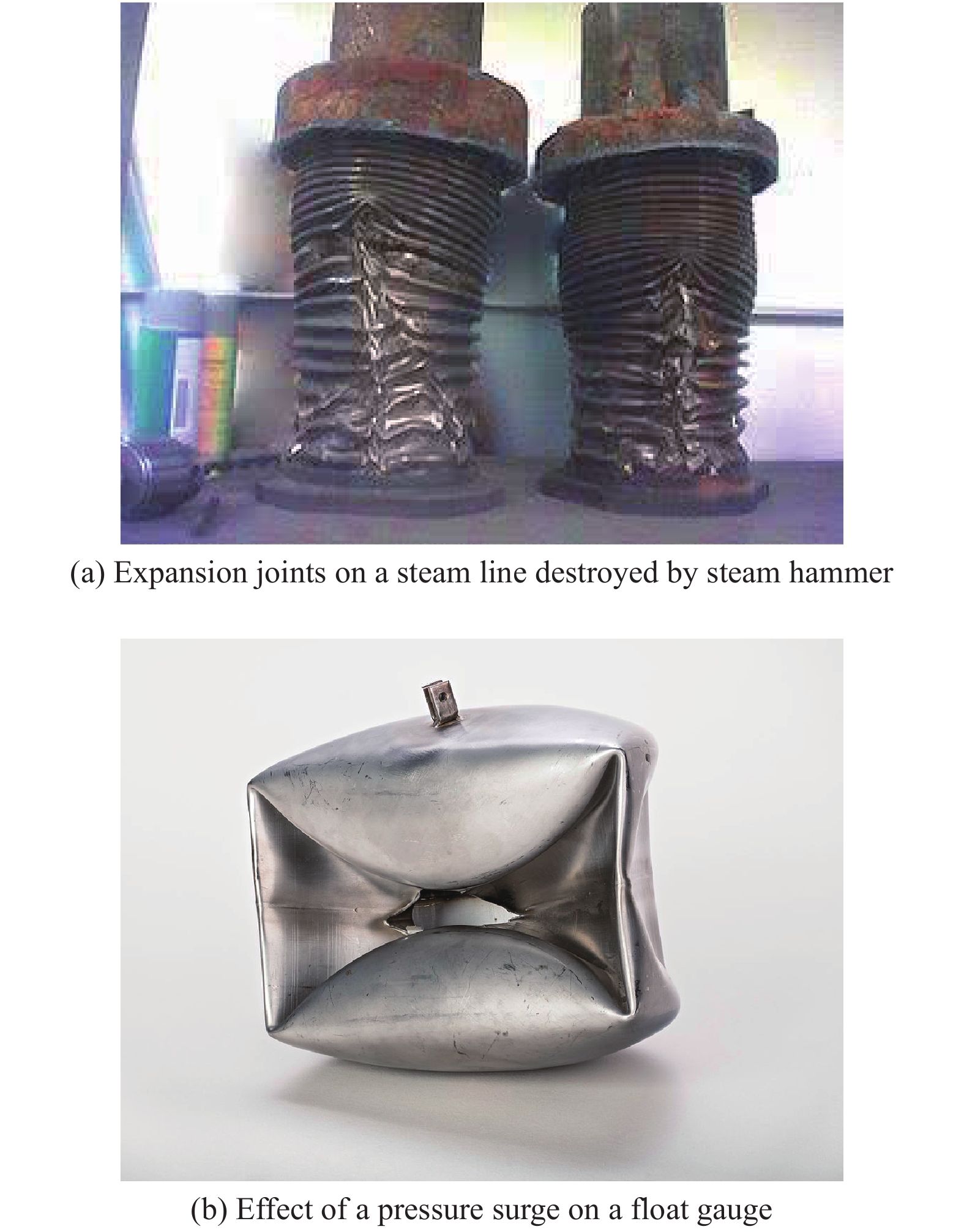
Examples of pipeline damage caused by hydraulic shock (Source: https://en.wikipedia.org/wiki/Water hammer)
 Volume 6
Issue 4
Volume 6
Issue 4
IEEE/CAA Journal of Automatica Sinica
| Citation: | Tehuan Chen and Zhigang Ren, "Optimal Valve Closure Operations for Pressure Suppression in Fluid Transport Pipelines," IEEE/CAA J. Autom. Sinica, vol. 6, no. 4, pp. 1010-1018, July 2019. doi: 10.1109/JAS.2019.1911585

|
HYDRAULIC shock phenomenon is a pressure surge or shock which commonly occurs when pipeline valves are manipulated in large-scale facilities for fluid distributions [1]. It generates pressure waves that propagate in the pipeline system at a high speed with a significant pressure oscillation, inducing harmful effects on the hydraulic facilities (examples of pipeline damage are shown in Fig. 1). Numerous pipeline collapses have occurred, such as pipelines leakage [2] and equipment failure of spacecraft propulsion systems [3], leading to loss of properties and even lives.
Numerous methods for solving hydraulic shock model which consists of hyperbolic PDEs can be divided into three categories: graphical methods, analytical methods, and numerical methods. The former two methods require many simplifying assumptions and mostly focus on the linear pipeline transmission PDE model. They especially cannot deal with the cavitation caused by negative pressure [4]. Although these two methods are very straightforward and simple, their applications are greatly limited in the real world. Numerical methods for simulating the hydraulic shock process mainly include methods of characteristics, finite volume methods, wave characteristics methods, impulse response methods, fluid-structure interaction methods [5], and even some computational packages (e.g., COMSOL Multiphysics, FINICS, etc.). In this paper, the method of lines is used for the reduction the hydraulic shock PDEs to time varying ODEs, which is easier to understand and implement compared with other methods. Then, the ODE system is approximated through the orthogonal collocation method to obtain a spatial-temporal discretization model (larger algebraic equations). Finally, the original PDE-constrained optimization problem reduces to a nonlinear programming problem, which can be solved with many existing high-quality optimization solvers, such as sequential quadratic programming (SQP).
To protect a pipeline system from hydraulic shock effects, various protection strategies can be employed, including passive protection and active control strategies. For passive protection strategies, specialized devices are set up to enhance the ability to resist pressure shock or reduce changes in the flow rate as much as possible. For instance, material and thickness of the pipeline that can be altered to withstand high pressure shocks [6]. Pipeline networks are designed by appropriate procedures (e.g., arranging the larger pipelines in loops that supply shorter and smaller run-out pipeline branches). Water towers (generally used in many drinking water systems) help maintain steady flow rates and trap large pressure fluctuations. Other pipeline equipments, such as surge tanks, air chamber, and non-return valves, are installed for precautions against pressure shock [7]. However, these strategies described above strongly depend on the specific details of each pipeline system and on the experience of the designer. Once the design of the pipeline system and structure is complete, it is still incapable of facing a variety of conditions during the operation of the pipeline due to lack of flexibility. Hence, advanced control strategies may be used as an alternative or as a supplement to various passive protection measures.
Mitigation of hydraulic shock can be considered as a PDE control problem. Generally, there are two categories of active control strategies for dealing with this problem: boundary stabilization control and optimal control [8], [9]. The boundary stabilization control can be divided into two streams of approaches based on their characteristic method, including the Lyapunov function method [10] and the backstepping technique [11]. For the Lyapunov function method, a boundary feedback control design for open canal networks is proposed in [12], where the stabilizing boundary control law is developed by linearizing the boundary conditions. A Lyapunov function is constructed based on the weighted sum of entropies for the open channels in cascade [13]. Global stability of a version of the rotating Couette flow is examined by the sum-of-squares of polynomials approach [14]. The boundary feedback stabilization for hydraulic shock suppression is studied in [15], which can guarantee the asymptotic stability towards the steady state. For the backstepping technique, boundary stabilization for a quasilinear
Since the basic characteristics of pressure and fluid flow in the pipeline are nonlinear, nonuniform, and coupled with each other, it is difficult to establish a relationship between the valve action and the responses of the hydrodynamic variables from an optimal control point of view. An analytical expression for the rate of change of relative water head in the S-shaped region of a pumped-storage station is deduced based on a simplified mathematical model followed by a two-phase guide-vane closing scheme are proposed in [20]. Several valve closure strategies based on the known valve performance curve with unknown valve closure curve are explored in [21]. Hybrid logistic optimization of pump locations and operation based on the rainfall-runoff model and the nonlinear pump model in urban drainage systems are described in [22]. The slow unsteady-incompressible hydraulics of pressurized pipe networks are simulated and the corresponding controlled operations of the turning pumps on and off are discussed in [23]. With the advent of modern control theories and numerical methodologies, large nonlinear optimization has made the control solution of nonlinear pipeline fluid flow possible. An effective approach based on the dynamic optimization strategy can be applied to implement optimal boundary control of flows in pipelines. The control vector parameterization (CVP) method [24]–[27] for hydraulic shock suppression based on the optimize-then-discretize (OTD) method [28] and discretize-then-optimize (DTO) method [24], [29] is proposed. In the framework of the OTD method for CVP, gradient formula and the costate PDEs with optimality conditions are derived directly via the variational method based on original PDEs. However, the convergence of the OTD method for CVP is blank. Moreover, the gradients of the time-scaling terms are very complicated and computational accuracy is hard to guarantee. In the framework of the DTO method for CVP, although the convergence analysis for ODEs is complete, the CVP method and time-scaling method leads to the iterative computation cost for solving the larger scale sensitivity equations (ODE equations), which is time consuming. In practice, we should design the control strategy as soon as possible when facing hydraulic shock. Thus, in order to speed up optimization efficiency and maintain certain calculation accuracy, we focus on optimal boundary control for pressure suppression in the pipeline system via a full parameterization (FP) method [30], which may have advantages in real-time. To our best knowledge, this work is seldom studied, and offers great promise in pressure suppression of fluid transport pipelines.
The main contributions of this paper are summarized as follows: 1) A new PDE-constrained optimization for pressure suppression in fluid transport pipelines is studied. The results can further explore the applications in the pipeline network scheduling. 2) A FP control strategy based on the methods of lines and orthogonal collocation is applied to pressure suppression control. 3) Numerical simulations are carried out to validate that the FP method eliminates pressure shock effectively and costs less computation time compared with the control vector parameterization (CVP) method.
This paper is organized as follows. Section II introduces a hyperbolic PDE system for fluid flow dynamics and a valve closing model for actual valve action, and then proposes an optimal control problem for pressure suppression in the pipeline during the valve closure. Through the method of lines and the orthogonal collocation for spatial-temporal discretization, the PDE optimization problem for pressure suppression is reduced to an NLP problem in Section III. Then, a gradient-based optimization framework for solving the approximate problem, which can be solved through intrinsic subroutine FMINCON on MATLAB, is proposed. Section IV shows the effectiveness of the proposed method for pressure suppression from simulation results. Furthermore, we give the comparison between CVP method and FP method for solving this optimal control problem and find that the FP method costs less computation time. Finally, Section V concludes the paper with summary comments and suggestions for future research.
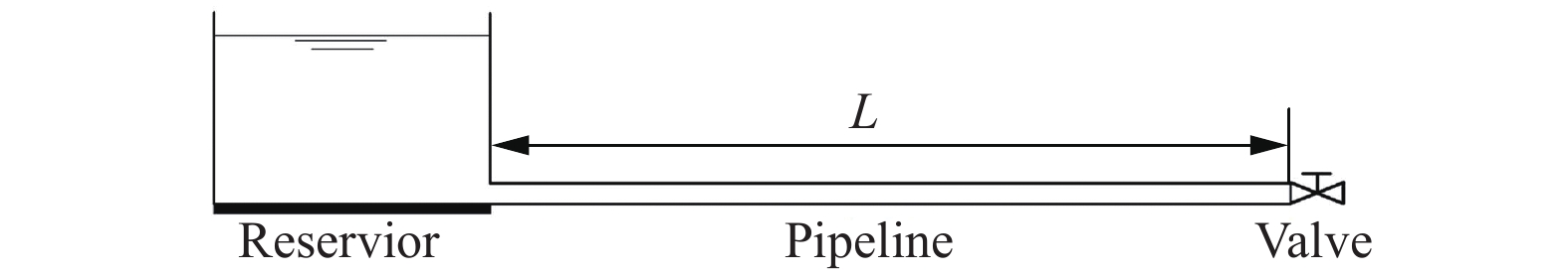
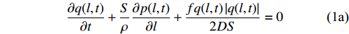
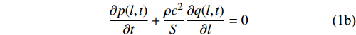
Consider the situation shown in Fig. 2, where a pipeline of length
|
∂q(l,t)∂t+Sρ∂p(l,t)∂l+fq(l,t)|q(l,t)|2DS=0 |
(1a) |
|
∂p(l,t)∂t+ρc2S∂q(l,t)∂l=0 |
(1b) |
subject to the boundary conditions
|
p(0,t)=P,q(L,t)=u(t),t∈[0,T] |
(2) |
where
Initially, the pipeline is in steady state during the operation process. Thus, the initial flow rate of the system (1) is
|
q(l,0)=Q,l∈[0,L] |
(3) |
where
|
p(l,0)=P−fρQ|Q|2DS2l,l∈[0,L]. |
(4) |
Moreover, a boundary control is required to satisfy the following bound constraint
|
0≤u(t)≤Umax,t∈[0,T] |
(5) |
where
|
u(T)=0. |
(6) |
Our interest lies in modeling the fluid flow along the pipeline during the valve closure period.
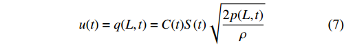
It is not the ultimate goal to get the curve of the terminal flow rate
We denote
|
u(t)=q(L,t)=C(t)S(t)√2p(L,t)ρ |
(7) |
where
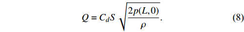
|
Q=CdS√2p(L,0)ρ. |
(8) |
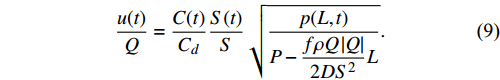
Based on (3) and (4), we divide (7) by (8) and obtain
|
u(t)Q=C(t)CdS(t)S√p(L,t)P−fρQ|Q|2DS2L. |
(9) |
Generally, the valve manufacturers provide the relationships between
| θ | α(t) | C(t)/Cd |
| 0 | 1 | 1 |
| 10 | 0.820 | 0.899 |
| 20 | 0.645 | 0.682 |
| 30 | 0.500 | 0.459 |
| 40 | 0.390 | 0.288 |
| 50 | 0.295 | 0.175 |
| 60 | 0.200 | 0.100 |
| 70 | 0.125 | 0.056 |
| 80 | 0.060 | 0.028 |
| 90 | 0.001 | 0.006 |
 DownLoad:
CSV
DownLoad:
CSV
Since the relationships between
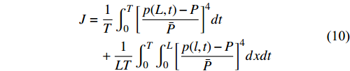
Since closing the valve suddenly can cause severe hydraulic shock effects, the boundary control
|
J=1T∫T0[p(L,t)−PˉP]4dt+1LT∫T0∫L0[p(l,t)−PˉP]4dxdt |
(10) |
where
Problem P0: Given the system (1a), (1b) with boundary conditions (2) and initial conditions (3), (4), choose the boundary control
In order to transfer the pipeline transmission PDE model into algebraic equations, we first use the method of lines to approximate the PDE model by an ODE model [36]. The total pipeline is divided into
|
qi(t)=q(li,t),pi(t)=p(li,t),i=0,…,NS. |
The
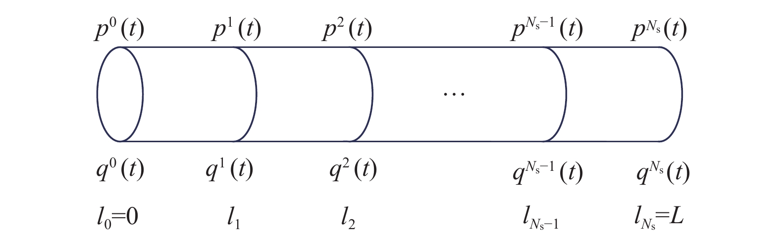
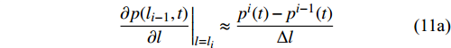
Based on the definitions of
|
∂p(li−1,t)∂l|l=li≈pi(t)−pi−1(t)Δl |
(11a) |
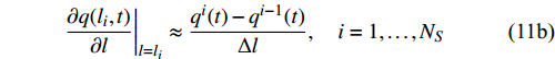
|
∂q(li,t)∂l|l=li≈qi(t)−qi−1(t)Δl,i=1,…,NS |
(11b) |
where
|
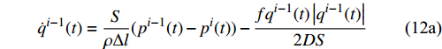
˙qi−1(t)=SρΔl(pi−1(t)−pi(t))−fqi−1(t)|qi−1(t)|2DS |
(12a) |
|
˙pi(t)=ρc2SΔl(qi−1(t)−qi(t)),i=1,…,NS. |
(12b) |
By virtue of the definitions of
|
p0(t)=P,qNS(t)=u(t),t∈[0,T]. |
(13) |
And (3), (4) can be written as
|
qi(0)=Q,pi(0)=P−fρQ|Q|2DS2li,i=0,1,…,NS. |
(14) |
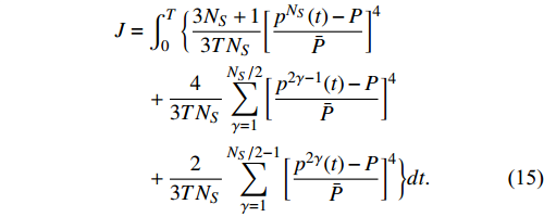
We apply the Simpson’s rule [37] to approximate (10) and obtain
|
J=∫T0{3NS+13TNS[pNS(t)−PˉP]4+43TNSNS/2∑γ=1[p2γ−1(t)−PˉP]4+23TNSNS/2−1∑γ=1[p2γ(t)−PˉP]4}dt. |
(15) |
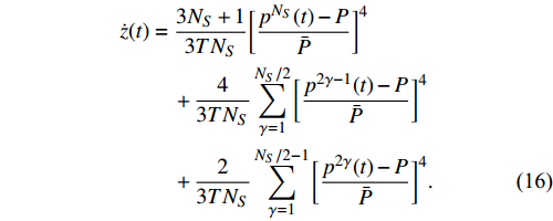
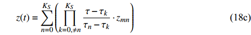
Since the objective function contains an integral form, we transfer it into a Mayer form by introducing a new state variable
|
˙z(t)=3NS+13TNS[pNS(t)−PˉP]4+43TNSNS/2∑γ=1[p2γ−1(t)−PˉP]4+23TNSNS/2−1∑γ=1[p2γ(t)−PˉP]4. |
(16) |
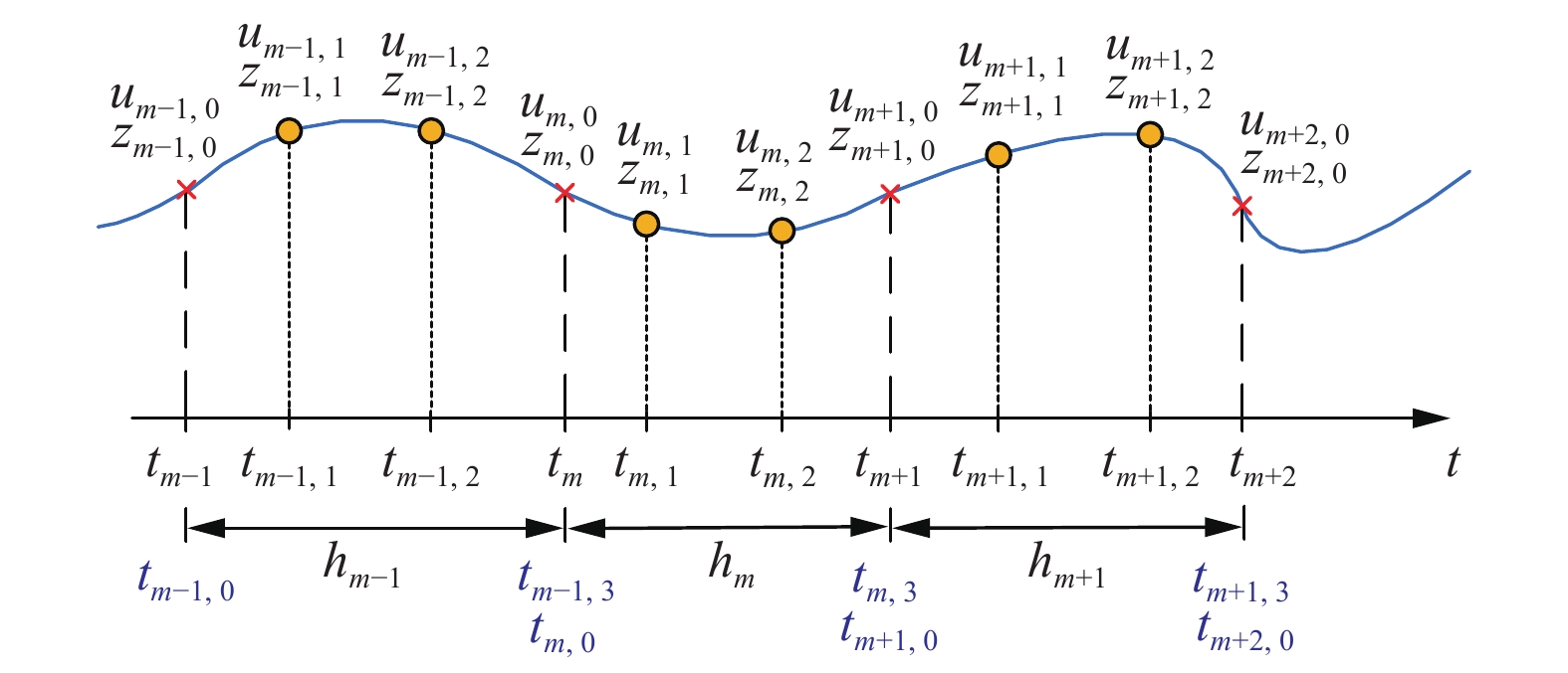
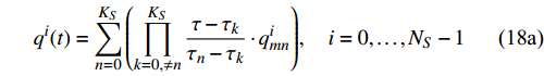
We approximate the ODEs through orthogonal collocation method, where those ODEs can be solved at selected points in the time domain. This method discretizes not only boundary control
First, the total time domain
|
t=tm+hmτ,t∈[tm,tm+1],τ∈[0,1] |
(17) |
where
|
qi(t)=KS∑n=0(KS∏k=0,≠nτ−τkτn−τk⋅qimn),i=0,…,NS−1 |
(18a) |
|
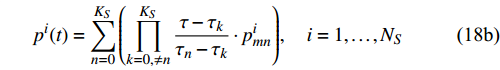
pi(t)=KS∑n=0(KS∏k=0,≠nτ−τkτn−τk⋅pimn),i=1,…,NS |
(18b) |
|
z(t)=KS∑n=0(KS∏k=0,≠nτ−τkτn−τk⋅zmn) |
(18c) |
where
|
u(t)=KU∑n=0(KU∏j=0,≠nτ−τjτn−τj⋅umj) |
(19) |
where
|
qim+1,0=KS∑n=0(KS∏k=0,≠n1−τkτn−τk⋅qimn)=qim,KS+1,i=0,…,NS−1 |
(20a) |
|
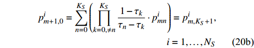
pim+1,0=KS∑n=0(KS∏k=0,≠n1−τkτn−τk⋅pimn)=pim,KS+1,i=1,…,NS |
(20b) |
|
zm+1,0=KS∑n=0(KS∏k=0,≠n1−τkτn−τk⋅zmn)=zm,KS+1 |
(20c) |
|
um+1,0=KU∑n=0(KU∏j=0,≠n1−τjτn−τj⋅umn)=um,KU+1 |
(20d) |
where
|
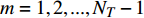
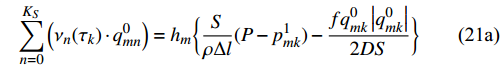
KS∑n=0(νn(τk)⋅q0mn)=hm{SρΔl(P−p1mk)−fq0mk|q0mk|2DS} |
(21a) |
|
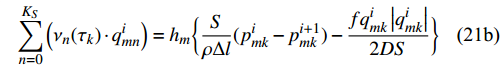
KS∑n=0(νn(τk)⋅qimn)=hm{SρΔl(pimk−pi+1mk)−fqimk|qimk|2DS} |
(21b) |
|
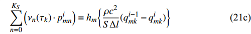
KS∑n=0(νn(τk)⋅pimn)=hm{ρc2SΔl(qi−1mk−qimk)} |
(21c) |
|
KS∑n=0(νn(τk)⋅pNSmn)=hm{ρc2SΔl(qNS−1mk−ωm(τk))} |
(21d) |
where
|
ωm(τk)={umk,KU=KSum(τk),KU<KS |
(22) |
and
|
KS∑n=0(νn(τk)⋅zmn)=hm{3NS+13TNS[pNSmk−PˉP]4+43TNSNS2∑γ=1[p2γ−1mk−PˉP]4+23TNSNS2−1∑γ=1[p2γmk−PˉP]4} |
(23) |
where
|
νn(τk)=d{KS∏k=0,≠nτ−τkτn−τk}dτ|τ=τk |
(24) |
and
|
i=1,…,NS−1,m=1,2,…,NT,k=1,2,…,KS. |
The initial conditions (14) become
|
qi1,0=Q,pi1,0=P−fρQ|Q|2DS2li,i=0,1,…,NS. |
(25) |
The control constraint (5) should be bounded at each time subintervals. Thus, it can be written as
|
0≤umj≤Umax,m=1,2,…,NT,j=1,…,KU |
(26) |
and the terminal control constraint (6) changes to
|
uNT,KU+1=KU∑n=0(KU∏j=0,≠n1−τjτn−τj⋅uNTn)=0. |
(27) |
Moreover, the time subintervals should be satisfied with the following equality constraint
|
NT∑m=1hm=T. |
(28) |
Finally, the objective function becomes
|
J=zNT,KS+1. |
(29) |
Remark 1: When
Problem PN: Given the algebraic system (21) and (23) with initial conditions (25), choose a control parameter vector
The approximate problem P
We give the main steps for solving the approximate problem P
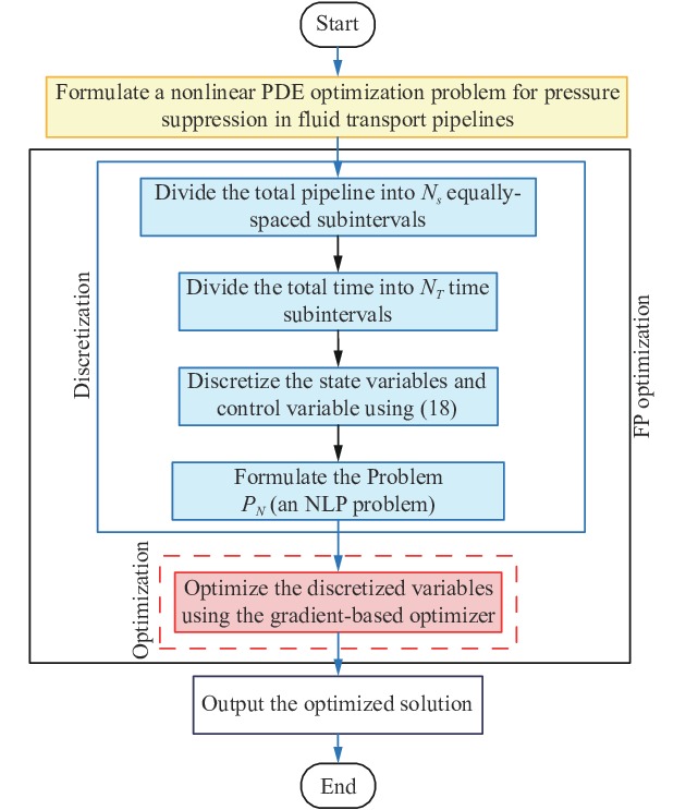
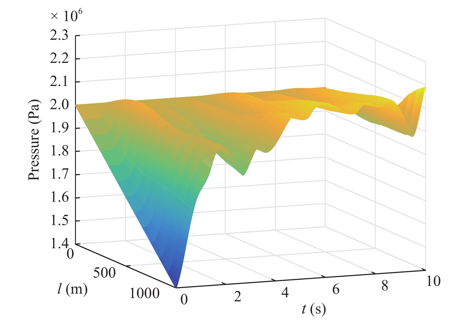
For the simulation, FP method with piecewise-linear control is applied for pressure suppression in fluid transport pipelines. The pipeline parameters are given as: the total pipeline length
We set
Our numerical simulation study was carried out within the MATLAB programming environment running on a personal computer with the following configuration: Intel (R) Core (TM) i5-2320 CPU, 3.00 GHz CPU, 4.00 GB RAM, 64-bit Windows 7 Operating System, MATLAB version is R2010b. Our MATLAB code implements the gradient-based optimization procedure in Fig. 5 via the intrinsic subroutine FMINCON of MATLAB.
The initial guess for the boundary control is chosen as
| Method | NS | CPU time (s) | Objective value |
| FP | 8 | 396 | 4.829 ×10⁻³ |
| CVP | 624 | 4.694 ×10⁻³ | |
| FP | 10 | 547 | 4.772 ×10⁻³ |
| CVP | 954 | 4.571 ×10⁻³ | |
| FP | 12 | 768 | 4.643 ×10⁻³ |
| CVP | 1459 | 4.458 ×10⁻³ |
DownLoad:
CSV
| m | hm | m | hm |
| 1 | 0.7031 | 6 | 0.6313 |
| 2 | 0.6995 | 7 | 1.9160 |
| 3 | 1.2866 | 8 | 1.0457 |
| 4 | 0.6484 | 9 | 1.1537 |
| 5 | 1.3853 | 10 | 0.5301 |
DownLoad:
CSV

In the case study, we use the intrinsic subroutine FMINCON of MATLAB to complete FP method on the optimal boundary control problem for pressure suppression since these two methods can be performed in this software platform. Readers may wonder whether the computation time is long. There are several methods to improve the computation efficiency. For example, we have transferred the optimization problem of the pipeline PDE system for pressure suppression into an NLP problem. This NLP problem could be solved by some specialized softwares very effectively, such as AMPL, GAMS combined with optimizer tool (e.g., IPOPT, SNOPT), which can greatly reduce the computation time.
Although this NLP problem can be effectively solved by certain specialized software, the computation is not cheap enough for real-world applications, which may not meet requirements of real-time optimization. Thus, a real-time implementation that takes less computation and execution time should be designed. A more effective method to improve the real-time performance is to built databases which record many optimal solutions under different physical parameters. Solution to the closest recorded case is extracted from the database and utilized as the on-site initial guess in practical applications. We test the computation cost under a suboptimal initial guess, which shows the optimal result can be obtained in around 9s on MATLAB. Of course, this result is not comprehensive and sufficient. Moreover, inspired by the operation of the beam pumping units [38], [39], the aim of this paper is to apply the proposed method into practice, we will study in the future.
This paper has presented an FP method for solving the PDE optimal control problem during valve closure periods towards pressure suppression. This method is based on a combination of the spatial discretization use the method of lines and time discretization by the orthogonal collocation method. The simulation results demonstrate the FP method is superior to the CVP method in terms of computation time. The simulation results demonstrate that the proposed method is effective toward pressure suppression. Since real-time implementation is more practical in the real-work by suitable scheduling of the valve operation sequences, the databases which record many optimal solutions under different physical parameters should be effectively built. Moreover, an improved predictive control strategy, dynamic programming with guaranteed satisfaction of path constraints, and a multi-objective optimization method for the nonlinear dynamic optimization are considered in [40]–[42], which can be extended to the spatial-temporal hydraulic shock model. These directions will be explored in future work.
| [1] |
M. Zhao and X. Sun, " Singular value decomposition-based collocation spectral method for quasi-two-dimensional laminar water hammer problems,” J. Hydraulic Engineering, vol. 143, no. 7, pp. 04017014, 2017. doi: 10.1061/(ASCE)HY.1943-7900.0001298
|
| [2] |
C. Xu, Y. Dong, Z. Ren, H. Jiang, and X. Yu, " Sensor deployment for pipeline leakage detection via optimal boundary control strategies,” J. Industrial and Management Optimization, vol. 11, no. 1, pp. 199–216, 2015.
|
| [3] |
C. Bombardieri, T. Traudt, and C. Manfletti, " Experimental and numerical analysis of water hammer during the filling process of pipelines,” in Space Propulsion, Jan. 2014.
|
| [4] |
Q. Yankai, L. Baoren, F. Xiaoyun, Y. Gang, and H. Junhua, " Suppressing water hammer of ship steering systems with hydraulic accumulator,” in Proc. Institution of Mechanical Engineers, Part E: J. Process Mechanical Engineering, 2013.
|
| [5] |
A. Keramat, A. S. Tijsseling, Q. Hou, and A. Ahmadi, " Fluid-structure interaction with pipe-wall viscoelasticity during water hammer,” J. Fluids and Structures, vol. 28, pp. 434–455, 2012. doi: 10.1016/j.jfluidstructs.2011.11.001
|
| [6] |
A. Adamkowski, S. Henclik, W. Janicki, and M. Lewandowski, " The influence of pipeline supports stiffness onto the water hammer run,” European J. Mechanics-B/Fluids, vol. 61, pp. 297–303, 2017. doi: 10.1016/j.euromechflu.2016.09.010
|
| [7] |
T. Larsen, Water Hammer in Pumped Sewer Mains. Aalborg University Press, 2012.
|
| [8] |
B. Luo, D. Liu, H. Wu, D. Wang, and F. L. Lewis, " Policy gradient adaptive dynamic programming for data-based optimal control,” IEEE Trans. Cybernetics, vol. 47, no. 10, pp. 3341–3354, 2017. doi: 10.1109/TCYB.2016.2623859
|
| [9] |
Z. Zhou, C. Yu, and K. L. Teo, " Some new results on integral-type backstepping method for a control problem governed by a linear heat equation,” IEEE Trans. Automatic Control, vol. 62, no. 7, pp. 3640–3645, 2017. doi: 10.1109/TAC.2017.2671778
|
| [10] |
W. He, C. Sun, and S. S. Ge, " Top tension control of a flexible marine riser by using integral-barrier Lyapunov function,” IEEE-ASME Trans. Mechatronics, vol. 20, no. 2, pp. 497–505, 2015. doi: 10.1109/TMECH.2014.2331713
|
| [11] |
M. Krstic and A. Smyshlyaev, Boundary Control of PDEs: A Course on Backstepping Designs. SIAM, 2008.
|
| [12] |
L. Cen, Y. Xi, D. Li, and Y. Cen, " Boundary feedback control of open canals with a Riemann invariants approach,” Trans. Institute of Measurement and Control, vol. 37, no. 7, pp. 900–908, 2015. doi: 10.1177/0142331213512365
|
| [13] |
L. Cen and Y. Xi, " Stability of boundary feedback control based on weighted Lyapunov function in networks of open channels,” Acta Autom. Sinica, vol. 35, no. 1, pp. 97–102, 2009.
|
| [14] |
D. Huang, S. Chernyshenko, P. J. Goulart, D. Lasagna, O. R. Tutty, and F. Fuentes, " Sum-of-squares of polynomials approach to nonlinear stability of fluid flows: an example of application,” Proce. Royal Society A:Mathematical,Physical and Engineering Sciences, vol. 471, no. 2183, pp. 20150622, 2015. doi: 10.1098/rspa.2015.0622
|
| [15] |
G. Bastin and J. M. Coron, Stability and Boundary Stabilization of 1-D Hyperbolic Systems. Springer International Publishing, 2016.
|
| [16] |
J. M. Coron, R. Vazquez, M. Krstic, and G. Bastin, " Local exponential H2 stabilization of a 2 × 2 quasilinear hyperbolic system using backstepping,” SIAM J. Control and Optimization, vol. 51, no. 3, pp. 2005–2035, 2013. doi: 10.1137/120875739
|
| [17] |
A. Diagne, M. Diagne, S. Tang, and M. Krstic, " Backstepping stabilization of the linearized saint-venant-exner model,” Automatica, vol. 76, pp. 345–354, 2017. doi: 10.1016/j.automatica.2016.10.017
|
| [18] |
T. V. Pham, D. Georges, and G. Besancçon, " Receding horizon boundary control of nonlinear conservation laws with shock avoidance,” Automatica, vol. 48, no. 9, pp. 2244–2251, 2012. doi: 10.1016/j.automatica.2012.06.025
|
| [19] |
X. Litrico and V. Fromion, " Boundary control of linearized Saint-Venant equations oscillating modes,” Automatica, vol. 42, no. 6, pp. 967–972, 2006. doi: 10.1016/j.automatica.2006.02.002
|
| [20] |
W. Zeng, J. Yang, J. Hu, and J. Yang, " Guide-vane closing schemes for pump-turbines based on transient characteristics in S-shaped region,” J. Fluids Engineering, vol. 138, no. 5, pp. 051302, 2016. doi: 10.1115/1.4032069
|
| [21] |
O. Skulovich, P. L. Sela, and A. Ostfeld, " Optimal closure of system actuators for transient control: an analytical approach,” J. Hydroinformatics, vol. 18, no. 3, pp. 393–408, 2016. doi: 10.2166/hydro.2015.121
|
| [22] |
Y. Cui, S. Hou, D. Li, Y. Xi, and L. Cen, " The optimization of location and control of pump stations in urban drainage system, ” in Proc. Chinese Control Conf., Chengdu, China, 2016.
|
| [23] |
J. Nault and B. Karney, " Improved rigid water column formulation for simulating slow transients and controlled operations,” J. Hydraulic Engineering, vol. 142, no. 9, pp. 04016025, 2016. doi: 10.1061/(ASCE)HY.1943-7900.0001145
|
| [24] |
T. Chen, Z. Ren, C. Xu, and R. Loxton, " Optimal boundary control for water hammer suppression in fluid transmission pipelines,” Computers &Mathematics with Applications, vol. 69, no. 4, pp. 275–290, 2015.
|
| [25] |
Z. Ren, C. Xu, Q. Lin, R. Loxton, and K. L. Teo, " Dynamic optimization of open-loop input signals for ramp-up current profiles in tokamak plasmas,” Communications in Nonlinear Science and Numerical Simulation, vol. 32, pp. 31–48, 2016. doi: 10.1016/j.cnsns.2015.08.005
|
| [26] |
Z. Ren, T. Chen, and Z. Wu, " Optimal matching control of a low energy charged particle beam in particle accelerators,” IEEE/CAA J. Autom. Sinica, vol. 6, no. 2, pp. 460–470, 2019. doi: 10.1109/JAS.6570654
|
| [27] |
Z. Ren, Z. Zhou, C. Xu, Z. Wu, and T. Chen, " Computational bilinear optimal control for a class of one-dimensional MHD flow systems,” ISA Trans., vol. 85, pp. 129–140, 2019. doi: 10.1016/j.isatra.2018.10.029
|
| [28] |
T. Chen and C. Xu, " Computational optimal control of the Saint-Venant PDE model using the time-scaling technique,” Asia-Pacific J. Chemical Engineering, vol. 11, no. 1, pp. 70–80, 2016. doi: 10.1002/apj.v11.1
|
| [29] |
T. Chen and Z. Ren, " Control of water hammer suppression via timescaling technique,” Control Theory and Applications, vol. 35, no. 2, pp. 198–206, 2018.
|
| [30] |
L. T. Biegler, Nonlinear Programming: Concepts, Algorithms, and Applications to Chemical Processes. Society for Industrial and Applied Mathematics, 2010.
|
| [31] |
M. S. Ghidaoui, " On the fundamental equations of water hammer,” Urban Water J., vol. 1, no. 2, pp. 71–83, 2004. doi: 10.1080/15730620412331290001
|
| [32] |
G. He, Y. Liang, Y. Li, M. Wu, L. Sun, C. Xie, and F. Li, " A method for simulating the entire leaking process and calculating the liquid leakage volume of a damaged pressurized pipeline,” J. Hazardous Materials, vol. 332, pp. 19–32, 2017. doi: 10.1016/j.jhazmat.2017.02.039
|
| [33] |
E. B. Wylie, V. L. Streeter, and L. Suo, Fluid Transients in Systems. Prentice Hall, Englewood Cliffs, 1993.
|
| [34] |
K. Yoshida and T. Ishikawa, " Flood hydrograph estimation using an adjoint shallow-water model,” J. Hydro-environment Research, vol. 9, no. 3, pp. 429–440, 2015. doi: 10.1016/j.jher.2014.12.003
|
| [35] |
T. Chen, C. Xu,, Q. Lin, R. Loxton, and K. L. Teo, " Water hammer mitigation via PDE-constrained optimization,” Control Engineering Practice, vol. 45, pp. 54–63, 2015. doi: 10.1016/j.conengprac.2015.08.008
|
| [36] |
W. E. Schiesser, Method of Iines PDE Analysis in Biomedical Science and Engineering. John Wiley & Sons, 2016.
|
| [37] |
D. Greenspan, Numerical Analysis. CRC Press, 2018.
|
| [38] |
K. Li and Y. Han, " Modelling for motor load torque with dynamic load changes of beam pumping units based on a serial hybrid model,” Trans. Institute of Measurement and Control, vol. 40, no. 3, pp. 903–917, 2018. doi: 10.1177/0142331216670454
|
| [39] |
K. Li, Y. Han, and T. Wang, " A novel prediction method for down-hole working conditions of the beam pumping unit based on 8-directions chain codes and online sequential extreme learning machine,” J. Petroleum Science and Engineering, vol. 160, pp. 285–301, 2018. doi: 10.1016/j.petrol.2017.10.052
|
| [40] |
Z. Tian, S. Li, and Y. Wang, " The multi-objective optimization model of flue aimed temperature of coke oven,” J. Chemical Engineering of Japan, vol. 51, no. 8, pp. 683–694, 2018. doi: 10.1252/jcej.17we159
|
| [41] |
J. Fu, J. M. Faust, B. Chachuat, and A. Mitsos, " Local optimization of dynamic programs with guaranteed satisfaction of path constraints,” Automatica, vol. 62, pp. 184–192, 2015. doi: 10.1016/j.automatica.2015.09.013
|
| [42] |
Z. Tian, S. Li, Y. Wang, and X. Wang, " SVM predictive control for calcination zone temperature in lime rotary kiln with improved pso algorithm,” Trans. Institute of Measurement and Control, vol. 40, no. 10, pp. 3134–3146, 2018. doi: 10.1177/0142331217716983
|
| [1] | Qinglai Zhang, Jianmin Gao, Qing Wu, Qinglie He, Libin Tie, Wanming Zhai, Shengyang Zhu. A Novel Vibration-Based Self-Adapting Method to Acquire Real-Time Following Distance for Virtually Coupled Trains[J]. IEEE/CAA Journal of Automatica Sinica, 2025, 12(1): 27-39. doi: 10.1109/JAS.2024.124326 |
| [2] | Xian-Ming Zhang, Qing-Long Han, Xiaohua Ge, Bao-Lin Zhang. Accumulative-Error-Based Event-Triggered Control for Discrete-Time Linear Systems: A Discrete-Time Looped Functional Method[J]. IEEE/CAA Journal of Automatica Sinica, 2025, 12(4): 683-693. doi: 10.1109/JAS.2024.124476 |
| [3] | Shulei Zhang, Runda Jia. A Self-Healing Predictive Control Method for Discrete-Time Nonlinear Systems[J]. IEEE/CAA Journal of Automatica Sinica, 2025, 12(4): 668-682. doi: 10.1109/JAS.2024.124620 |
| [4] | Ying Chen, Feilong Lin, Zhongyu Chen, Changbing Tang, Cailian Chen. Optimal Production Capacity Matching for Blockchain-Enabled Manufacturing Collaboration With the Iterative Double Auction Method[J]. IEEE/CAA Journal of Automatica Sinica, 2025, 12(3): 550-562. doi: 10.1109/JAS.2024.124626 |
| [5] | Han Xu, Jiayi Ma, Yixuan Yuan, Hao Zhang, Xin Tian, Xiaojie Guo. More Than Lightening: A Self-Supervised Low-Light Image Enhancement Method Capable for Multiple Degradations[J]. IEEE/CAA Journal of Automatica Sinica, 2024, 11(3): 622-637. doi: 10.1109/JAS.2024.124263 |
| [6] | Zhaohui Jiang, Chuan Xu, Jinshi Liu, Weichao Luo, Zhiwen Chen, Weihua Gui. A Dual Closed-Loop Digital Twin Construction Method for Optimizing the Copper Disc Casting Process[J]. IEEE/CAA Journal of Automatica Sinica, 2024, 11(3): 581-594. doi: 10.1109/JAS.2023.123777 |
| [7] | Yong-Chao Li, Rui-Sheng Jia, Ying-Xiang Hu, Hong-Mei Sun. A Weakly-Supervised Crowd Density Estimation Method Based on Two-Stage Linear Feature Calibration[J]. IEEE/CAA Journal of Automatica Sinica, 2024, 11(4): 965-981. doi: 10.1109/JAS.2023.123960 |
| [8] | Zhongcai Zhang, Guangren Duan. Stabilization Controller of An Extended Chained Nonholonomic System With Disturbance: An FAS Approach[J]. IEEE/CAA Journal of Automatica Sinica, 2024, 11(5): 1262-1273. doi: 10.1109/JAS.2023.124098 |
| [9] | Zongyu Zuo, Jingchuan Tang, Ruiqi Ke, Qing-Long Han. Hyperbolic Tangent Function-Based Protocols for Global/Semi-Global Finite-Time Consensus of Multi-Agent Systems[J]. IEEE/CAA Journal of Automatica Sinica, 2024, 11(6): 1381-1397. doi: 10.1109/JAS.2024.124485 |
| [10] | Sheng Cao, Zhiwei Luo, Changqin Quan. Sequential Inverse Optimal Control of Discrete-Time Systems[J]. IEEE/CAA Journal of Automatica Sinica, 2024, 11(3): 608-621. doi: 10.1109/JAS.2023.123762 |
| [11] | Yang Li, Xiao Wang, Zhifan He, Ze Wang, Ke Cheng, Sanchuan Ding, Yijing Fan, Xiaotao Li, Yawen Niu, Shanpeng Xiao, Zhenqi Hao, Bin Gao, Huaqiang Wu. Industry-Oriented Detection Method of PCBA Defects Using Semantic Segmentation Models[J]. IEEE/CAA Journal of Automatica Sinica, 2024, 11(6): 1438-1446. doi: 10.1109/JAS.2024.124422 |
| [12] | Min Yang, Guanjun Liu, Ziyuan Zhou, Jiacun Wang. Probabilistic Automata-Based Method for Enhancing Performance of Deep Reinforcement Learning Systems[J]. IEEE/CAA Journal of Automatica Sinica, 2024, 11(11): 2327-2339. doi: 10.1109/JAS.2024.124818 |
| [13] | Zheng Chen, Shizhao Zhou, Chong Shen, Litong Lyu, Junhui Zhang, Bin Yao. Observer-Based Adaptive Robust Precision Motion Control of a Multi-Joint Hydraulic Manipulator[J]. IEEE/CAA Journal of Automatica Sinica, 2024, 11(5): 1213-1226. doi: 10.1109/JAS.2024.124209 |
| [14] | Feiye Zhang, Qingyu Yang, Dou An. Privacy Preserving Demand Side Management Method via Multi-Agent Reinforcement Learning[J]. IEEE/CAA Journal of Automatica Sinica, 2023, 10(10): 1984-1999. doi: 10.1109/JAS.2023.123321 |
| [15] | Zhe Chen, Ning Li. An Optimal Control-Based Distributed Reinforcement Learning Framework for A Class of Non-Convex Objective Functionals of the Multi-Agent Network[J]. IEEE/CAA Journal of Automatica Sinica, 2023, 10(11): 2081-2093. doi: 10.1109/JAS.2022.105992 |
| [16] | Fanghui Bi, Xin Luo, Bo Shen, Hongli Dong, Zidong Wang. Proximal Alternating-Direction-Method-of- Multipliers-Incorporated Nonnegative Latent Factor Analysis[J]. IEEE/CAA Journal of Automatica Sinica, 2023, 10(6): 1388-1406. doi: 10.1109/JAS.2023.123474 |
| [17] | Jingbei Yang, Shuang Cong, Feng Shuang, Herschel Rabitz. Manipulations Between Eigenstates of 2-Level Quantum System Based on Optimal Measurements[J]. IEEE/CAA Journal of Automatica Sinica, 2016, 3(1): 35-41. |
| [18] | Mingxiang Dai, Ying He, Xinmin Yang. Continuous-time System Identification with Nuclear Norm Minimization and GPMF-based Subspace Method[J]. IEEE/CAA Journal of Automatica Sinica, 2016, 3(2): 184-191. |
| [19] | Xiaojun Tang, Jie Chen. Direct Trajectory Optimization and Costate Estimation of Infinite-horizon Optimal Control Problems Using Collocation at the Flipped Legendre-Gauss-Radau Points[J]. IEEE/CAA Journal of Automatica Sinica, 2016, 3(2): 174-183. |
| [20] | Qiming Zhao, Hao Xu, Sarangapani Jagannathan. Near Optimal Output Feedback Control of Nonlinear Discrete-time Systems Based on Reinforcement Neural Network Learning[J]. IEEE/CAA Journal of Automatica Sinica, 2014, 1(4): 372-384. |

Figures(7) / Tables(3)


Tehuan Chen and Zhigang Ren, "Optimal Valve Closure Operations for Pressure Suppression in Fluid Transport Pipelines," IEEE/CAA J. Autom. Sinica, vol. 6, no. 4, pp. 1010-1018, July 2019. doi: 10.1109/JAS.2019.1911585
| θ | α(t) | C(t)/Cd |
| 0 | 1 | 1 |
| 10 | 0.820 | 0.899 |
| 20 | 0.645 | 0.682 |
| 30 | 0.500 | 0.459 |
| 40 | 0.390 | 0.288 |
| 50 | 0.295 | 0.175 |
| 60 | 0.200 | 0.100 |
| 70 | 0.125 | 0.056 |
| 80 | 0.060 | 0.028 |
| 90 | 0.001 | 0.006 |
DownLoad:
CSV
| Method | NS | CPU time (s) | Objective value |
| FP | 8 | 396 | 4.829 ×10⁻³ |
| CVP | 624 | 4.694 ×10⁻³ | |
| FP | 10 | 547 | 4.772 ×10⁻³ |
| CVP | 954 | 4.571 ×10⁻³ | |
| FP | 12 | 768 | 4.643 ×10⁻³ |
| CVP | 1459 | 4.458 ×10⁻³ |
DownLoad:
CSV
| m | hm | m | hm |
| 1 | 0.7031 | 6 | 0.6313 |
| 2 | 0.6995 | 7 | 1.9160 |
| 3 | 1.2866 | 8 | 1.0457 |
| 4 | 0.6484 | 9 | 1.1537 |
| 5 | 1.3853 | 10 | 0.5301 |
DownLoad:
CSV
| θ | α(t) | C(t)/Cd |
| 0 | 1 | 1 |
| 10 | 0.820 | 0.899 |
| 20 | 0.645 | 0.682 |
| 30 | 0.500 | 0.459 |
| 40 | 0.390 | 0.288 |
| 50 | 0.295 | 0.175 |
| 60 | 0.200 | 0.100 |
| 70 | 0.125 | 0.056 |
| 80 | 0.060 | 0.028 |
| 90 | 0.001 | 0.006 |
| Method | NS | CPU time (s) | Objective value |
| FP | 8 | 396 | 4.829 ×10⁻³ |
| CVP | 624 | 4.694 ×10⁻³ | |
| FP | 10 | 547 | 4.772 ×10⁻³ |
| CVP | 954 | 4.571 ×10⁻³ | |
| FP | 12 | 768 | 4.643 ×10⁻³ |
| CVP | 1459 | 4.458 ×10⁻³ |
| m | hm | m | hm |
| 1 | 0.7031 | 6 | 0.6313 |
| 2 | 0.6995 | 7 | 1.9160 |
| 3 | 1.2866 | 8 | 1.0457 |
| 4 | 0.6484 | 9 | 1.1537 |
| 5 | 1.3853 | 10 | 0.5301 |
 DownLoad:


 DownLoad:


