Surrogate-Assisted Particle Swarm Optimization Algorithm With Pareto Active Learning for Expensive Multi-Objective Optimization

I. Introduction

MULTI-OBJECTIVE optimization problems are co mmonly encountered in real world [1], e.g., drug design [2], aerodynamic configuration optimization [3] and hyper-parameter optimization for machine learning models [4]. However, the analytic objective or constraints functions in the above cases are difficult to express accurately. Thus, it is a challenge to implement the optimization only based on data collected from physical experiments, real events, or complex numerical simulations [5]. In these cases, it is essential to obtain the desired outcome within a small number of evaluations. Generally, the multi-objective optimization problem can be generalized as follows:

where ${{x}}\in\mathbb{R}^{n}$ represents a vector of $n$ decision variables; $S\subset\mathbb{R}^{n}$ indicates the feasible region which is typically specified as a set of constraints on the decision variables; ${{f}}\in\mathbb{R}^{m}$ is made of $m$ objective functions which need to be jointly minimized; ${{y}}$ is an $m$-dimensional objective vector.

Considering the high convergence speed and simple implementation, multi-objective particle swarm optimization (MOPSO) attracts great attention which gives rise to a series of variants in the existing literature [6]. Generally, they can be classified into two categories. One is based on the Pareto sorting strategy [7]–[9], and the other employs the decomposition strategy [10], [11]. Although the variants of MOPSO algorithm above have been proved to be with the satisfactory convergence, they require thousands of fitness evaluations to obtain satisfied solutions. As a result, applying MOPSO on computationally expensive problems becomes impractical when a single exact fitness evaluation exhibits a high computational cost. To enhance the performance of most traditional PSOs in solving multi-objective optimization problems, a number of approaches have been proposed [12].

Surrogate-assisted PSO algorithms (SAPSOs) have be found very effective in handling computationally expensive multi-objective optimization problems [13], [14]. Some employ single or multiple surrogates to approximate the fitness function. For instance, a study presented in [15] took use of a response surface model (RSM) rather than finite-element analysis. The Kriging model is applied to gain error compensation function between the approximated values obtained by RSM and the actual measured values in [16]. While others typically estimates the degree of uncertainty to choose certified candidates for re-evaluation, e.g., the Kriging model was combined with MOPSO method to predict the expected improvements of each particle in [17]. Reference [18] captured the uncertainty with the hypervolume to pre-select promising particles for re-evaluation. All of the above studies have shown the effectiveness of SAPSO on reducing the number of fitness function evaluations.

Furthermore, as indicated in [5], [14], surrogate model management is critical for the performance of SAPSOs [19]. A typical strategy is to employ the generation-based method, in which the expensive fitness evaluations are replaced by computationally cheap approximating models [20]. But it is not practical for many extremely expensive problems because a large number of expensive fitness evaluations were needed for an accurate surrogate model [14]. Another known as individual-based model management focus on the determination of individuals demanding evaluation for each generation. Three criteria, such as minimizing the predicted fitness [21], minimizing the prediction uncertainty [18] and a combination of the previous two [22] are normally used to select new candidate solutions to be evaluated. However, it is difficult to strike a proper balance between exploration and exploitation [19]. Besides, active learning (AL) is a commonly deployed alternative for model management. In such a case, the new training data are actively queried for efficiently improving the approximation quality of the current model without significantly increasing the size of training dataset. Also, AL terminates when any additional training data have no effect on the information gain [23].

As already shown in [24], AL-based methods can also be used for solving the multi-objective optimization problem. For example, an active learning method of the Pareto front was reported in [23], in which a surrogate model was constructed to approximate the Pareto front. A PSO assisted by the active learning method based on the committee was presented in [19], but it only considered the single objective problem with the high computational cost. In [25], a Pareto active learning (PAL) method was proposed to predict the Pareto optimal solutions. In comparison to the state-of-the-art algorithm PAL, a $\varepsilon$-Pareto active learning ($\varepsilon$-PAL) was presented in [26] to reduce computational complexity. However, how to select $\varepsilon$ for achieving a satisfied tradeoff between prediction accuracy and classification cost is a challenge.

In this paper, we assume that the optimization algorithm is allowed to evaluate a small number of selected solutions during optimization. It should be noted that we focus on developing a surrogate-assisted PSO with Pareto active leaning so as to effectively accelerate the convergence process. The main contributions of this work can be highlighted as follows:

1) A mixed mutation sampling method based on simulated evolution is proposed to enhance the quality of the candidate solutions. Based on the advantage of fast convergence of PSO, the evolution of the swarm is simulated with the surrogate model rather than the true fitness function. And the particles which are beyond the Pareto front and locate at the sparse part of the Pareto front are carried out the mutation operation to promote the diversity of the population. Then the positions of the offspring are considered as the candidate solutions.

2) A classification strategy using the improved $\varepsilon$-PAL is employed to identify candidate solutions that are Pareto-optimal and not Pareto-optimal. It is wellknown that the prediction accuracy and classification cost are controlled by parameter $\varepsilon$. However, the mathematical relationship between parameter $\varepsilon$, prediction accuracy and classification cost are not clear. This poses a challenge for determining the value of $\varepsilon$. Therefore, a greedy search method is suggested to select $\varepsilon$ where the number of active sampling is employed as the evaluation criteria of the classification cost.

3) A surrogate-assisted PSO with Pareto active learning is proposed to solve the computationally expensive optimization problems with multiple objectives. The Pareto-optimal solutions obtained by $\varepsilon$-PAL are used to guide the global search of the swarm, while the history information of PSO is employed to update the surrogate models.

The rest of this paper is organized as follows. Section II presents a brief introduction to PSO, Gauss process modeling and $\varepsilon$-PAL. Then, a surrogate-assisted PSO with Pareto active learning is proposed in Section III. In Section IV, the results obtained from the numerical studies on eight benchmark test problems and two MLSSVM model optimization problems with the proposed algorithm are discussed. Finally, Section V draws the conclusions for this study.

II. Preliminaries

A Particle Swarm Optimization

PSO [27] adopts experiences from both individuals and swarms to guide the direction of evolution. Assuming the population size is known as $NP$, the velocity and the location of the $i\mathrm{th}$ particle at $t$ generation are updated as follows:

where $\omega$ indicates the inertia weight; $c_{1}$ and $c_{2}$ are the learning rate; $r_{1}$ and $r_{2}$ represent the random numbers which are belong to $(0, 1)$; ${{p}}_{i}(t)$ and ${{p}}_{g}(t)$ stand for the personal best and the global best at $t$ generation, respectively.

B Gaussian Process Modelling

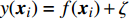
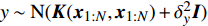
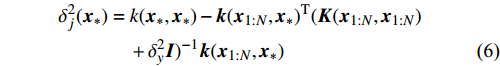
Gauss process (GP) [28] surrogate model is employed to approximate each objective. For the $j\mathrm{th}$ objective, the response function is expressed as $y({{x}}_{i}) = f({{x}}_{i})+\zeta$, where $f({{x}}_{i})$ indicates the mapping function between the input ${{x}}_{1:N}$ and the output $y_{1:N}$; $\zeta\sim{ {\rm {N}}}(0, \delta^2_{y})$ denotes the Gaussian noise. With the GP prior, the response function of the $j\mathrm{th}$ objective is formulated as $y\sim{ {\rm {N}}}({{K}}({{x}}_{1:N}, {{x}}_{1:N})+\delta^2_{y}{{I}})$. Given the new point ${{x}}_{\ast}$, the mean $\mu_{j}({{x}}_{\ast})$ and variance $\delta^2_{j}({{x}}_{\ast})$ are expressed as follows:

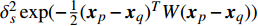
where $\mu_{j}$ and $\delta^2_{j}$ indicate the predicted mean value and variance for the $j\mathrm{th}$ objective, respectively; ${{K}}$ denotes the covariance matrix using the squared exponential function $k({{x}}_{p}, {{x}}_{q}) =$$\delta^2_{s}\exp(-\frac{1}{2}({{x}}_{p}-{{x}}_{q})^T{{W}}({{x}}_{p}-{{x}}_{q}))$, where $\delta^2_{s}$ represents the signal variance and ${{W}}$ is the widths of the kernel.

C $\varepsilon$-Pareto Active Learning

The $\varepsilon$-PAL [26] method is a classification method which is utilized to find $\varepsilon$-accurate Pareto front with as few function evaluations as possible. In $\varepsilon$-PAL, GP models are adopted to predict the candidate solutions that have not been evaluated yet. Furthermore, the predictive uncertainty is employed to guide the iterative sampling. Specifically, the sampling strategy is designed to maximize the probability that candidate solutions are Pareto-optimal. With a set of classification rules, the candidate solutions are identified as the Pareto-optimal and non-Pareto-optimal solutions with high probability. At last, $\varepsilon$-PAL terminates when all the candidate solutions are classified. The computing procedures for $\varepsilon$-PAL are summarized as Algorithm 1.

Algorithm 1 The framework of $\varepsilon$-PAL

Input: $U_{i}$ (undecided points), $P_{i}$ (predicted set), $\varepsilon$ (user-controlled parameter)

1: Initialize $U_{1}=E$, $P_{1}= \emptyset$ and set $i=1$.

2: while $U_{i}\neq \emptyset$ do

3: Construct the surrogate model for each objective using (5) and (6).

4: Assign the uncertainty region $R_{i}({{x}})$ for each point ${{x}}\in U_{i}\cup P_{i}$.

5: Discard the points in $U_{i}$ which are $\varepsilon$-dominated by another point with high probability.

6: Move the points that belong to the $\varepsilon$-Pareto front of $E$ from $U_{i}$ to $P_{i}$.

7: Sample a point from $U_{i}\cup P_{i}$.

8: $i=i+1$.

9: end while

Output: $\varepsilon$-accurate Pareto set $\widehat{P}=P_{i}$.

 | Show Table

DownLoad: CSV

III. The Proposed Surrogate-Assisted PSO Algorithm With Pareto Active Learning

A The Overall Framework

In this paper, the evaluation of the fitness function is considered to be computationally expensive. In order to obtain Pareto optimal solutions with the limited number of the fitness evaluations, a novel surrogate-assisted PSO with the help of Pareto active learning, termed PAL-SAPSO, is proposed in this section.

The pseudo code of PAL-SAPSO is given as Algorithm 2, which can be summarized as six procedures as follows:

1) Initialization (line 1): $NP$ particles are generated using Latin hypercube sampling, which are evaluated using the fitness function. Then the external archive and the knowledge base are initialized.

2) Swarm update (line 3 to 4): The swarm is updated with the personal best and the global best.

3) Construction of surrogate model (line 7): The surrogate model is built with data in the knowledge base to approximate the fitness function for each objective.

4) Sampling of candidate solution set (line 8): The mixed mutation sampling method based on the simulated evolution is implemented to get the candidate solutions.

5) Classification of candidate solution set (line 9): The improved $\varepsilon$-PAL is employed to categorize the candidate solutions into Pareto-optimal solutions and non-Pareto-optimal ones.

6) Update of the external archive (line 10): The external archive is updated by pre-selecting results from the improved $\varepsilon$-PAL.

7) Repeat Step 2) to Step 6) until the maximum number of fitness evaluations is reached.

In PAL-SAPSO, the sampling method and the classification strategy are crucial for the success of the algorithm. We will discuss them in detail in the following subsections.

Algorithm 2 The framework of PAL-SAPSO

Input: $NP$ (population size), ${v}$ (velocity), ${x}$ (position), $A$ (external archive), $D_{t}$ (knowledge base with $N_{t}$ samples at $t$ generation), $N_{\max}$ (maximum number of the fitness evaluations).

1: Initialize $NP$, ${{v}}$, ${{x}}$, $A$, $D_{t}$ and set $N_{t}=NP$.

2: while $N_{t} \le N_{\max}$ do

3: Select the personal best ${{p}}_{i}(t)$ and the global best ${{p}}_{g}(t)$.

4: Update ${{v}}(t)$ and ${{x}}(t)$ using (3) and (4), and calculate the corresponding fitness ${{f}}({{x}})$.

5: Update $A$ (Using Algorithm 5).

6: Update $D_{t}$ with $\{{{x}}, {{f}}({{x}})\}$.

7: Construct the surrogate model for each objective using (5) and (6).

8: Get the candidate solution set (Using Algorithm 3).

9: Get the $\varepsilon$-accurate Pareto optimal solution set (Using Algorithm 4).

10: Update $A$ (Using Algorithm 5).

11: Update $D_{t}$.

12: Count the number of the fitness evaluations $N_{t}$.

13: $t=t+1$.

14: end while

Output: Pareto-optimal solutions from $A$.

 | Show Table

DownLoad: CSV

B A Hybrid Mutation Sampling Method Based on the Simulated Evolution

For maintaining convergence and diversity of the candidate solutions, a hybrid mutation sampling method based on simulated evolution is proposed. The main framework of the sampling method is listed in Algorithm 3.

1) Simulated Evolution of the Particle Swarm: The PSO algorithm tries to find the optimal solution using a population of particles. Based on (3) and (4), it is clear that the trajectories drawn by the particles are semi-random in nature, as they derive from the contribution of systematic attraction towards the personal and global best solutions and the stochastic weighting of two acceleration terms [27]. Furthermore, PSO is known to have a very high convergence speed. Inspired by the above ideas, a sampling method based on the simulated evolution is designed to obtain the candidate solutions.

Let us assume that the population of the $t\mathrm{th}$ generation in the real physical space is migrated into the virtual space where the cheap surrogate models are employed to take place of the computationally expensive fitness functions. Then the information of the initial population is expressed as ${{x}}^{\prime}_{i}(1) = {{x}}_{i}(t)$, ${{v}}^{\prime}_{i}(1) = {{v}}_{i}(t)$, $\widehat{{{p}}}_{i}(1) = {{p}}_{i}(t)$, $\widehat{{{p}}}_{g}(1) = {{p}}_{g}(t)$ and $\widehat{A}(1) = {A}(t)$. With the initial information, the velocity and position of each particle are updated as follows:

where ${{v}}^{\prime}_{i}(k)$ and ${{x}}^{\prime}_{i}(k)$ indicate the velocity and the position of the $i\mathrm{th}$ particle in the virtual space at the $k\mathrm{th}$ iteration in the virtual space. $\widehat{{{p}}}_{i}(k)$ and $\widehat{{{p}}}_{g}(k)$ denote the personal best and the global best of the swarm at the $k\mathrm{th}$ iteration in the virtual space; $\widehat{A}$ and $A$ are the external archives in the virtual space and the real physical space, respectively.

In the process of simulated evolution, the surrogate models based on GP are used to replace the real fitness function. Based on the experience knowledge base $D_{t} = \{{{x}}_{i}, y_{i, j}|1\leq i \leq$$N_{t}, 1\leq j\leq m\}$, $m$ surrogate models are constructed for $m$ objectives. Given any position of particle ${{x}}^{\prime}_{i}$, fitness is estimated by $\widehat{{{y}}}_{i} = (\mu_{1}({{x}}^{\prime}_{i}), \ldots , \mu_{m}({{x}}^{\prime}_{i}))$, where $\mu_{j}(\cdot)$ represents the estimated value of the $j\mathrm{th}$ surrogate model. Then the personal best and the global best are updated as presented in Section III-D.

2) Mutation on Particles Beyond the Pareto Front: Although particles which float away from the Pareto front are useful for maintaining the diversity of the population, they will slow down the convergence speed. In addition, non-dominant solutions are usually required to be as close as possible to the real Pareto front. Therefore, the mutation operation moving the particles towards to the Pareto front can not only accelerate the convergence speed, but also improve the quality of the solution.

The particles which are beyond the Pareto front are identified first. The approximate Pareto front corresponding to the non-dominant solutions in the external archive is used as the reference front because of the real Pareto front is usually unknown. In the object space, the Euclidean distances between the fitness values of the particles and the reference front are different. Then, the particles whose Euclidean distance is larger than the average distance are considered to be far from the Pareto front, as expressed in the following formula:

where $O$ denotes the set of the particles which are far from the Pareto front; ${{x}}^{\prime}$ indicates the position of the particle which beyond the Pareto front; $l_{i}$ indicates the Euclidean distance between the fitness values of the $i\mathrm{th}$ particle and the closest non-dominant solution; $\bar{l}$ is the mean of $l_{i}$; $find(\cdot)$ represents the query function on the index of the element; $\widehat{A}(k)$ stands for the external archive at the $k\mathrm{th}$ iteration in the virtual space; $\widehat{{{y}}}_{i}$ indicates the estimated values of the fitness of $i\mathrm{th}$ particle; ${{a}}_{j}$ denotes the fitness values of the non-dominant solutions on the Pareto front.

Let ${{x}}^{\prime}_{i}$ is the particle beyond the Pareto front, then the mutation operation is carried out as follows:

where ${{x}}^{\prime \prime}_{i}(k)$ indicates the new position of the $i\mathrm{th}$ particle in the virtual space at the $k\mathrm{th}$ iteration; ${{x}}^{\ast}_{i}$ denotes the closest non-dominant solution to ${{x}}^{\prime}$; $r\in\{0, 1\}$.

3) Mutation to Particles Locating at the Sparse Part of the Pareto Front: In the process of simulated evolution, a large number of particles will aggregate to the individual non-dominant solution according to the fast convergence of PSO. It causes that parts of Pareto front correspond to more non-dominant solutions, while others correspond to fewer. Then, the diversity distribution of the solutions becomes worse. Therefore, it is an effective method to identify the sparse parts of the Pareto front and generate new non-dominant solutions in the sparse parts.

First of all, the particles which locate at the sparse part of the Pareto front are identified. The Pareto front constructed by the non-dominant solutions in the external archive is also used as the reference front. For any objective, the fitness values of the non-dominant solutions in the external archive are arranged in ascending order and the Euclidean distance between two adjacent non-dominant solutions is computed. When the Euclidean distance of the two non-dominant solutions is larger than the average distance of all adjacent non-dominant solutions, the part between two non-dominant solutions is considered to be sparse according to the following formula:

where $S$ denotes the set of the sparse parts of the Pareto front; ${{x}}^{\ast}_{h}$ and ${{x}}^{\ast}_{h+1}$ represent the non-dominant solutions at the edge of the sparse part of the Pareto front; $d_{j}$ indicates the Euclidean distance of the two adjacent non-dominant solutions; $\bar{d}$ is the mean of $d_{j}$.

Let ${{x}}^{\ast}_{h}$ and ${{x}}^{\ast}_{h+1}$ denote the non-dominant solutions at the edge of the sparse part of the Pareto front. Then, both particles move towards each other. The mutation operation is formulated as

where ${{x}}^{\prime \prime \prime}(k)$ indicates the position of the new particle which locates at the sparse part of the Pareto front in virtual space at the $k\mathrm{th}$ iteration.

4) A Hybrid Mutation Sampling Strategy Based on the Simulated Evolution: In the process of the simulated evolution, the positions of the particles involving the offspring and the particles which are beyond the Pareto front and locate at the sparse part of the Pareto front are updated at each generation. To get more information on position in the search space, the swarm is simulated $\eta$ generations in virtual space. Then the candidate solutions obtained by mutation operation are determined as

where $X_{\rm pss}$ denotes the set of candidate solutions; ${{x}}^{\prime}$, ${{x}}^{\prime \prime}$ and ${{x}}^{\prime \prime \prime}$ indicate the candidate solutions which are obtained from three mutation operations, respectively.

Algorithm 3 A hybrid mutation sampling method based on the simulated evolution

Input: ${v}^{\prime}$ (velocity), ${x}^{\prime}$ (position), $\widehat{{p}}_{i}$ (personal best), $\widehat{{p}}_{g}$ (global best), $\widehat{A}$ (external archive), $\eta$ (maximum number of generations).

1: Initialize ${{v}}^{\prime}={{v}}$, ${{x}}^{\prime}={{x}}$, $\widehat{{{p}}}_{i}(1)={{{p}}}_{i}(t)$, $\widehat{{{p}}}_{g}(1)={{{p}}}_{g}(t)$, $\widehat{A}(1)=A(t)$.

2: for $k=1$ to $\eta$ do

3: Update ${{v}}^{\prime}(k)$ and ${{x}}^{\prime}(k)$ using (7) and (8).

4: Evaluate the fitness based on (5).

5: Determine the particles which are beyond Pareto front using (9) and (10), and obtain new particles ${{x}}^{\prime \prime}(k)$ based on (11).

6: Determine the particles which locate the sparse part of the Pareto front using (12) and (13), and obtain the new particles ${{x}}^{\prime \prime \prime}(k)$ based on (14).

7: Get the set of the candidate solution $X_{\rm pss}$ according to (15).

8: Update $\widehat{A}(k)$ with $\{X_{\rm pss}, \widehat{{{y}}}(X_{\rm pss})\}$.

9: Select the personal best $\widehat{{{p}}}_{i}(k)$ and the global best $\widehat{{{p}}}_{g}(k)$.

10: end for

Output: The candidate solution set $X_{\rm pss}$.

 | Show Table

DownLoad: CSV

C Classification Using Improved $\varepsilon$-Pareto Active Learning

In PAL-SAPSO, $\varepsilon$-PAL is employed to categorize the candidate solutions. Although the Pareto-optimal set obtained by $\varepsilon$-PAL is likely to be Pareto-optimal at current generation, but the candidate solutions can not cover the whole search space. As a result, the predicted Pareto-optimal set may not belong to the true Pareto front for the problem to be solved. Furthermore, the fitness function is computational expense, the classification cost from the sampling and the evaluations of the predicted Pareto-optimal solutions must be considered. In order to achieve a tradeoff between prediction accuracy and the classification cost, an improved $\varepsilon$-PAL is proposed, as described in Algorithm 4.

As suggested in [26], the $\varepsilon$-PAL automatically stops when the target accuracy $\varepsilon$ is achieved with confidence $1-\varpi$. Obviously, once the target accuracy $\varepsilon$ is fixed, there is a theoretical boundary for the sampling number. In turn, the target accuracy $\varepsilon$ can be obtained when the sampling number is given.

From line 7 in Algorithm 1, it is clear that each point in $U_{i}\cup P_{i}$ have the possibility of being sampled. Let the desired number of evaluations, $T$, is equal to the number of the points in $U_{i}\cup P_{i}$. Then, the prediction accuracy $\varepsilon$ is determined if the classification cost $T$ is given. In order to achieve a balance between prediction accuracy $\varepsilon$ and classification cost $T$, the resulting nonlinear programming problem can be expressed as follows:

where $n_{j}$ denotes the number of the points in $U_{i}\cup P_{i}$ at the $j\mathrm{th}$ greedy search; $\varepsilon_{l}$ and $\varepsilon_{u}$ represent the upper and lower bound of the target accuracy $\varepsilon$, respectively.

Taking (16) into account, it is apparent that satisfactory prediction accuracy can be found under the expected classification cost. As a result, a balance strategy is presented by solving (16) greedily in the following form:

where $\tau$ represents the learning factor, $\tau\in\{0, 1\}$; $\Delta$ denotes the speed of searching. Based on the balance strategy, a set of $\varepsilon$-accurate Pareto optimal solutions $\widehat{P}_{T}$ is obtained with the desired classification cost $T$.

Algorithm 4 The framework of improved $\varepsilon$-PAL

Input: $U_{i}$ (undecided points), $P_{i}$ (predicted set), $T\;$ (classification cost), $N_{\rm GS}$ (maximum number of greedy searches), $\tau$ (learning factor).

1: Initialize $U_{1}=X_{\rm pss}$, $P_{1}= \emptyset$, $\varepsilon\in [\varepsilon_{l}, \varepsilon_{u}]$, $U^{\prime}= \emptyset$, $P^{\prime}= \emptyset$ and set $i=1$

2: while $U_{i}\neq \emptyset$ do

3: Assign the uncertainty region $R_{i}({{x})$ for each point ${{x}\in U_{i}\cup P_{i}$

4: Discard the points in $U_{i}$ which are $\varepsilon$-dominated by another point with high probability.

5: Move the points that belong to the $\varepsilon$-Pareto front of $X_{\rm pss}$ from $U_{i}$ to $P_{i}$.

6: Count the number of the points $n_{1}$ in $U_{i}\cup P_{i}$.

7: Initialize $U^{\prime}_{1}=U_{i}$, $P^{\prime}_{1}=P_{i}$ and set $j=1$.

8: while $n_{j}>T$ or $j<N_{\rm GS}$ do

9: Assign the uncertainty region $R^{\prime}_{j}({{x}^{\prime})$ for each point ${{x}^{\prime}\in U^{\prime}_{j}\cup P^{\prime}_{j}$.

10: Determine the value of $\varepsilon$ using (17) to (19).

11: Discard the points in $U^{\prime}_{j}$ which are $\varepsilon$-dominated byanother point with high probability.

12: Move the points that belong to the $\varepsilon$-Pareto frontof $X_{\rm pss}$ from to $U^{\prime}_{j}$ $P^{\prime}_{j}$.

13: $j=j+1$.

14: Count the number of the points $n_{j}$ in $U^{\prime}_{j}\cup P^{\prime}_{j}$.

15: Save the value of $\varepsilon$.

16: end while

17: Sample a point from $U_{i}\cup P_{i}$.

18: $i=i+1$.

19: end while

Output: The $\varepsilon$-accurate Pareto set $\widehat{P}_{T}=P_{i}$.

 | Show Table

DownLoad: CSV

D Selection of Personal and Global Best Particle

For the multiobjective optimization problems, PSO intends to search for a set of non-dominated solutions to be stored in an external archive with a predefined size $N_{\rm rep}$. After initializing the PSO population, every particle will fly toward the direction guided by its personal best and global best. However, the PSO-based algorithm may converge to a false Pareto front because of its very high convergence speed. Therefore, it is important to ensure that the particles in the population move toward a more sparse and promising region in the search space.

At the $t\mathrm{th}$ generation, the personal best of the $i\mathrm{th}$ particle ${{p}}_{i}(t)$ is updated by a new solution ${{x}}_{i}(t+1)$ found by this particle if ${{p}}_{i}(t)$ is dominated by ${{x}}_{i}(t+1)$. And, the personal best of the $i\mathrm{th}$ particle is selected between ${{p}}_{i}(t)$ and ${{x}}_{i}(t+1)$ randomly if they are non-dominated with respect to each other.

The global best ${{p}}_{g}(t)$ is selected from the external archive randomly, which is useful in guiding the particle to fly in the different direction. In addition, the external archive is updated with the approximate Pareto solution set $\widehat{P}_{T}$ to enhance the social experience of the population, as described in Algorithm 5. Here, the popular archive update mechanism used in [6] is also adopted, which is based on both Pareto dominance and crowding distance.

Algorithm 5 Archive update

Input: $\widehat{P}_{T}$ ($\varepsilon$-accurate Pareto set), $A$ (external archive), $N_{\rm rep}$ (size of external archive)

1: for $i=1$ to $|\widehat{P}_{T}|$ do

2: if $\widehat{P}_{i}$ is dominated by any member in $A$ then

3: Discard $\widehat{P}_{i}$.

4: else if $\widehat{P}_{i}$ dominates a set of member in $A$ then

5: $A=A \cup \{\widehat{P}_{i}\}$.

6: else if $\widehat{P}_{i}$ and any member of $A$ are non-dominatedwith each other then

7: $A=A \cup \{\widehat{P}_{i}\}$.

8: end if

9: if $|A|$ $>$ $N_{\rm rep}$ then

10: Calculate the crowding distance value for each solution in $A$.

11: Delete the most crowed one.

12: end if

13: end for

Output: The external archive $A$.

 | Show Table

DownLoad: CSV

E Computational Complexity of One Generation of the Proposed Algorithm

The proposed algorithm in this study consists of a hybrid mutation sampling method based on simulated evolution, improved $\varepsilon$-PAL and PSO. Firstly, in the hybrid mutation sampling method based on simulated evolution, 1) implementation of PSO requires ${\rm{O}}(NP\times N^2_{\rm rep})$ computations. 2) Construction of the surrogate models require ${\rm{O}}(m\times N^3_{t})$ computations. 3) Assuming the number of candidate solutions is $N_{\rm pss} = (NP+N_{\rm rep})\times \eta$ (In fact, the number of candidate solutions is smaller than the hypothetical value because not all particles implement mutation). Thus, the estimation of the candidate solutions require ${\rm{O}}(N_{\rm pss}\times N^2_{t})$ computations. Due to $N_{t}$ increases dynamically, the worst-case complexity of the hybrid mutation sampling method based on simulated evolution is ${\rm{O}}(m\times N^3_{t})$. Secondly, in the improved $\varepsilon$-PAL, 1) determination of the value of $\varepsilon$ requires ${\rm{O}}(N_{\rm pss}{\rm log}(N_{\rm pss})\times$$N_{\rm GS})$ computations ($\varepsilon$-PAL requires ${\rm{O}}(n{\rm log}(n))$ computations on every iteration [26], where $n$ indicates the number of the undecided points), where $N_{\rm GS}$ is the number of greedy searches. 2) Identification of Pareto solutions require ${\rm{O}}$$(m\times (N_{t}+T-1)^3+(N_{t}+T-1)^2)$ computations (In the worst case, the active sampling is carried out $T$ times and $1{\rm log}(1) = 0$). Thus, considering the worst case, the complexity of the improved $\varepsilon$-PAL is ${\rm{O}}(m\times (N_{t}+T-1)^3+(N_{t}+T-1)^2)$. And finally, PSO optimizer requires ${\rm{O}}(NP\times N^2_{\rm rep})$ computations. Considering all the above computations, the overall worst-case complexity of generation of the proposed algorithm is ${\rm{O}}(m\times (N_{t}+T-1)^3+(N_{t}+T-1)^2)$.

IV. Experimental Studies

A Comparative Experiment on Benchmark Problems

To verify the performance of the proposed method (PAL-SAPSO), three existing MOPSO algorithms were employed to make a comparison with a set of widely used benchmark test problems. Three state-of-the-art MOPSO algorithms include standard MOPSO [27], decomposition-based multi-objective particle swarm optimization (dMOPSO) [29] and speed-constrained multi-objective PSO (SMPSO) [30]. Both dMOPSO and SMPSO are improved version of standard MOPSO. In addition, dMOPSO is based on decomposition strategy and SMPSO adopts Pareto sorting strategy. The source codes of three MOPSO algorithms are provided in PlatEMO [31]. All parameters are set to the recommended values in the original papers.

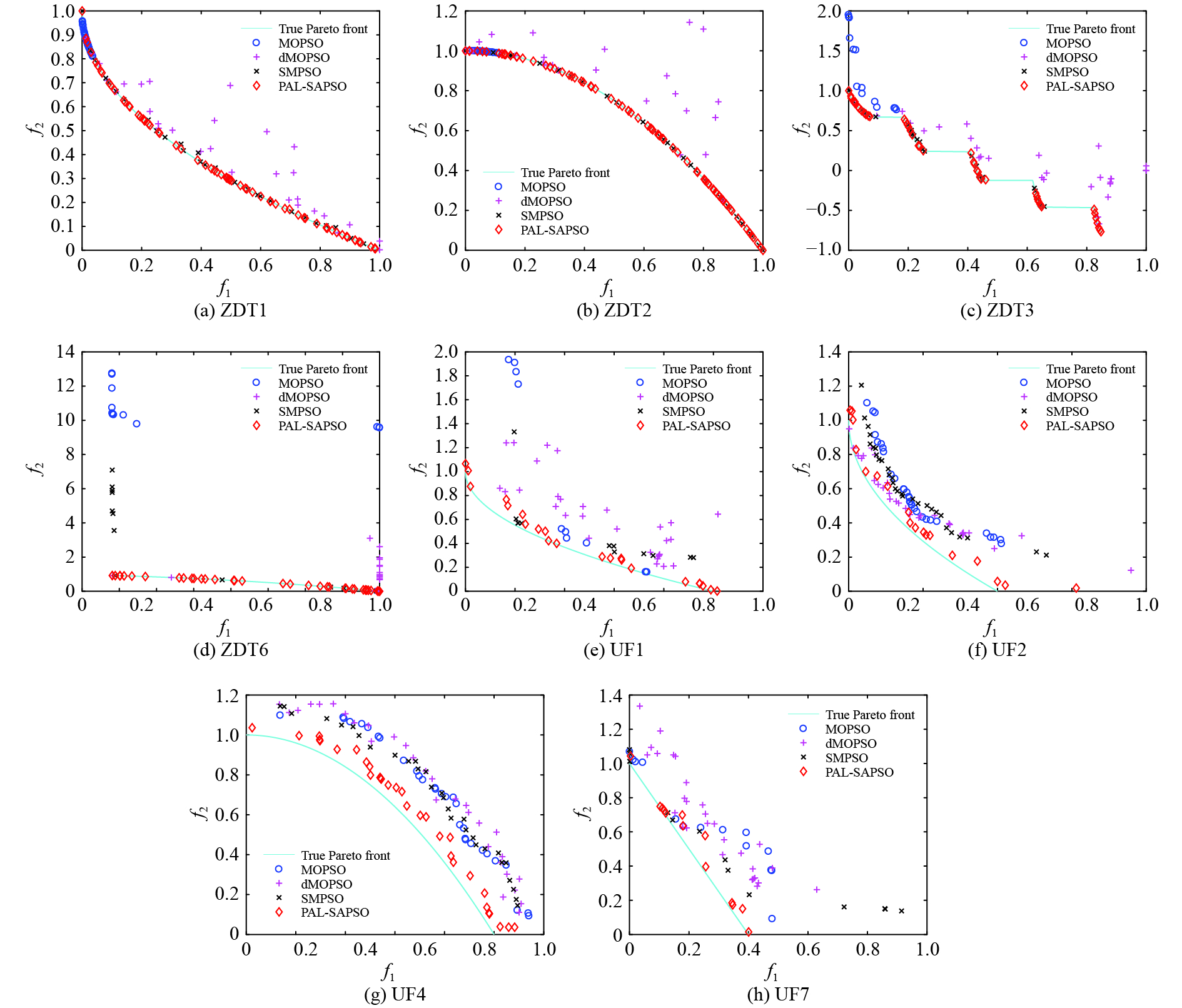
A total of 8 test problems with two objectives are used to evaluate the performance of the algorithms, where ZDT1, ZDT2, ZDT3, UF1, UF2, UF4 and UF7 have 6 decision variables and ZDT6 is 10. The mathematical description of the test problems was given in [32]. The inverted generational distance (IGD) metric [33] is deployed as the index for evaluating the performance of the compared algorithms, and almost 1000 points uniformly sampled on the Pareto front are used in the calculation of IGD for each test problem. The IGD is defined as follows:

where $P_{\rm true}$ represents the true Pareto front reference points; $P_{\rm rep}$ denotes the non-dominant solution in the external archive; $dis({{x}}, P_{\rm rep})$ denotes the Euclidean distance between ${{x}}$ and the non-dominant solution in the external archive; $|P_{\rm true}|$ is the number of real Pareto forward reference points. The IGD is a metric for evaluating the quality of obtained solution set in terms of both convergence and distribution. The smaller the IGD value, the better the quality of solution set obtained by the algorithm.

The parameters of the proposed algorithm PAL-SAPSO are set as follows: the population size is set to $NP = 30$; the inertia weight is set to $\omega = 0.5$; the learning rate is set to $c_{1} = 1$ and $c_{2} = 2$; the generation of the simulated evolutionary is set to $\eta = 20$; the learning factor is set to $\tau = 0.02$; the prediction accuracy is set to $\varepsilon\in \{0, 1\}$, the classification cost is set to $T = 5$ and the number of the greedy searches is set to $N_{\rm GS} = 1000$. For each test problem, 20 independent experiments are conducted and the maximum number of the fitness evaluations is set to 500, 1000, 1500 and 2000. All experimental results are obtained on a PC (with an Intel Core i5 6200U CPU) and MATLAB 2017a.

The comparative results from 4 algorithms (MOPSO, dMOPSO, SMPSO, and PAL-SAPSO) with 500 function evaluation on ZDT and UF test problems are showed in Table I. The statistical results consist of the mean (the corresponding standard deviation) of IGD which are obtained from 20 independent experiments. It can be seen from Table I that the mean of IGD from PAL-SAPSO is smaller than the other algorithms. It exhibits that the Pareto fronts obtained by PAL-SAPSO have the best performance on the convergence and the distribution. And, the standard deviation of the means from PAL-SAPSO are the smallest. It shows that PAL-SAPSO has good stability. To clearly visualize the comparison of results, the Pareto fronts which are obtained by 4 algorithms with 500 function evaluation on ZDT and UF test problems are illustrated in Fig. 1. The results in Fig. 1 correspond to the smallest values of IGD in the 20 independent experiments. It can be concluded that PAL-SAPSO effectively converges to the true front and find the more diverse solutions compared to MOPSO, dMOPSO and SMPSO.

Table  I.  Comparative Results From 4 MOPSO Algorithms

Problem	MOPSO	dMOPSO	SMPSO	PAL-SAPSO
ZDT1	3.86 (2.69)	3.39×10−1 (2.18×10−1)	6.87×10−1 (9.07×10−1)	1.21×10−2 (3.38×10−3)
ZDT2	3.60 (2.43)	5.52×10−1 (2.01×10−1)	6.26×10−1 (9.94×10−1)	4.45×10−2 (1.34×10−1)
ZDT3	2.70 (1.85)	3.21×10−2 (1.70×10−1)	5.36×10−1 (4.62×10−1)	2.90×10−2 (1.31×10−2)
ZDT6	1.06×10 (8.96×10−1)	5.04×10−1 (1.37×10−1)	8.14 (2.33)	4.80×10−2 (3.12×10−2)
UF1	2.79×10−1 (6.93×10−2)	2.93×10−1 (7.80×10−2)	2.70×10−1 (8.44×10−2)	6.68×10−2 (2.41×10−2)
UF2	2.13×10−1 (2.22×10−2)	1.71×10−1 (1.56×10−2)	2.11×10−1 (1.83×10−2)	1.15×10−1 (4.75×10−2)
UF4	1.93×10−1 (1.30×10−2)	1.88×10−1 (7.97×10−3)	1.74×10−1 (6.58×10−3)	6.69×10−2 (7.93×10−3)
UF7	3.87×10−1 (8.55×10−2)	3.39×10−1 (1.35×10−1)	1.74×10−1 (1.27×10−1)	1.34×10−1 (4.81×10−2)

 | Show Table

DownLoad: CSV

Figure  1.  The convergence results obtained by algorithms on 8 test problems.

DownLoad: Full-Size Img PowerPoint

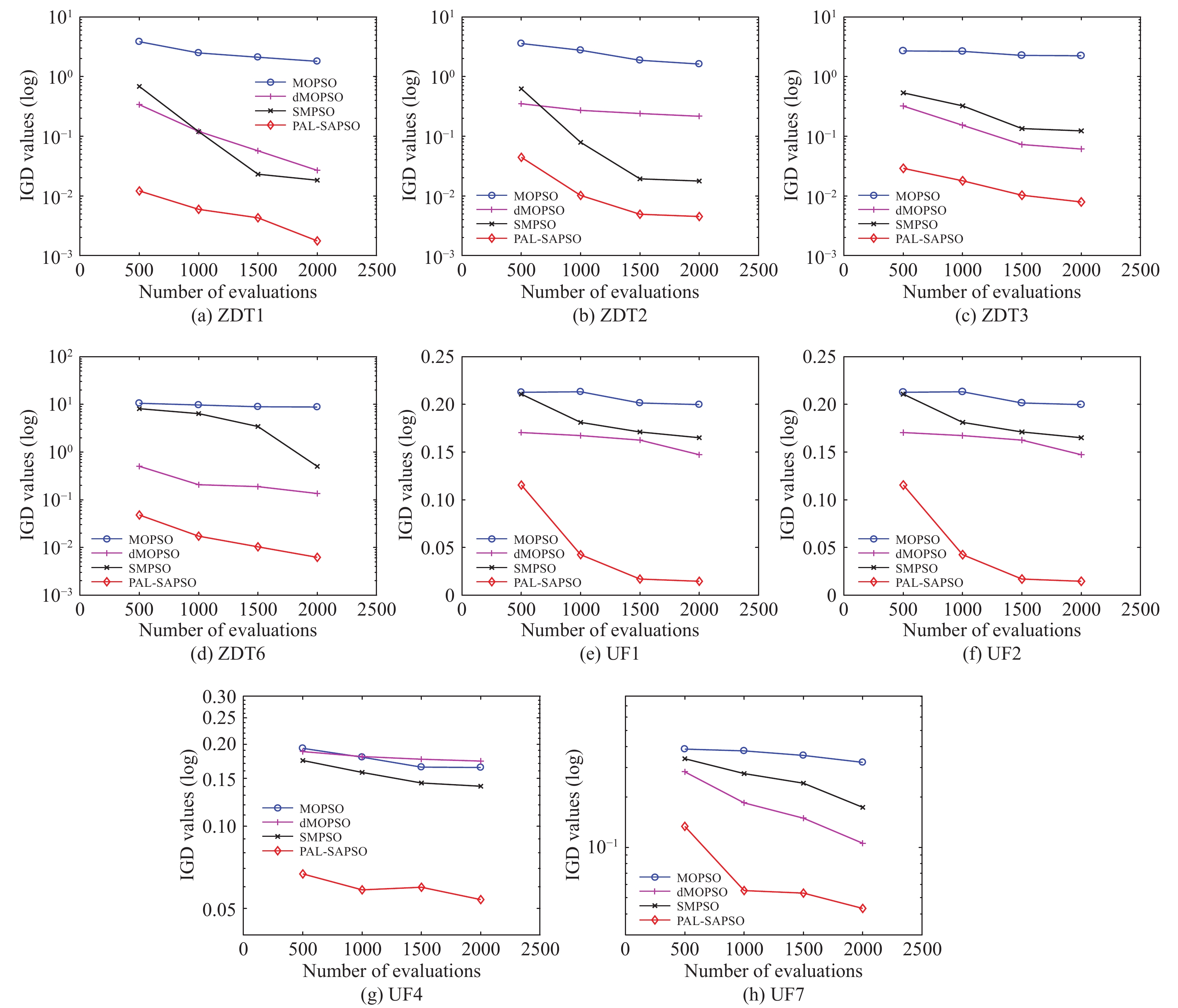
To further investigate the convergence of PAL-SAPSO, the mean of IGD from MOPSO, dMOPSO, SMPSO, and PAL-SAPSO on ZDT and UF test problems with the 500, 1000, 1500, and 2000 fitness evaluations are shown in Fig. 2. As shown in these figures, the convergence of PAL-SAPSO is better than MOPSO, dMOPSO and SMPSO.

Figure  2.  The convergence results obtained by algorithms on 8 test problems.

DownLoad: Full-Size Img PowerPoint

In summary, compared with MOPSO, dMOPSO and SMPSO, the Pareto fronts obtained by PAL-SAPSO have better performance on convergence and distribution with the same number of the fitness evaluations.

B Comparative Experiments on Parameter Determination for MLSSVM-based Model

In order to further verify the effectiveness of the proposed algorithm, two application problems arising from the parameter determination for MLSSVM-based models [34] are employed. In general, the generalization capability of the data-driven model is evaluated by the multifold cross-validation method [35].

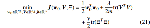
For predicting an output vector ${{y}}\in\mathbb{R}^{m}$ from a given input vector ${{x}}\in\mathbb{R}^{n}$, the MLSSVM-based model is established by solving a constraint-based optimization problem [34]

Once the Lagrangian function is constructed with respect to (21) and (22), a linear system is obtained with Karush-Kuhn-Tucker (KKT) conditions as follows:

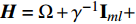
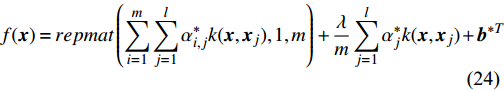
where ${{P}} = blockdiag({\bf{1}}_{l}, {\bf{1}}_{l}, \dots, {\bf{1}}_{l})\in \mathbb{R}^{ml\times m}$, ${{H}} = \Omega+\gamma^{-1}{\bf{I}}_{ml}+$$(m/ \lambda){{Q}}\in \mathbb{R}^{ml\times ml}$ is the positive definite matrix. If the solutions ($\alpha^{\ast}$ and ${{b}}^{\ast}$) of (23) are obtained, one can get the corresponding decision function for multiple outputs as follows:s

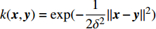
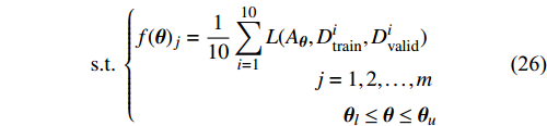
where $k({ x}, { y}) = {\rm exp}(-\dfrac{1}{2\delta^{2}}\|{ x}-{ y}\|^{2})$. Three parameters (two positive real regularized parameters $\lambda$, $\gamma$ and kernel parameter $\delta$) in MLSSVM model should be determined. In order to obtain a MLSSVM regression model with the satisfactory generalization, the 10-fold cross-validation method is adopted. The optimization problem is described as follows:

where ${{E}}$ represents the cross-validation error (the mean square error); $f({\theta})_{j}$ denotes the $j\mathrm{th}$ objective function; $A_{{\theta}}$ indicates the MLSSVM model with the parameters ${\theta} = (\lambda, \gamma, \delta)$; $L(A_{{\theta}},$$D_{\rm train}^{i}, D_{\rm valid}^{i})$ represents the cross-validation method; $D_{\rm train}^{i}$ stands for the training data; $D_{\rm valid}^{i}$ is the validation data; ${\theta}_{l}$ and ${\theta}_{u}$ denote the upper and lower boundaries of the parameters ${\theta}$, respectively.

To evaluate the effectiveness of the parameter configuration scheme, the predictive performance of the MLSSVM model is evaluated by the mean square error $MSE = \dfrac{1}{l}\displaystyle\sum\nolimits_{i = 1}^{l}(y_{i}-\widehat{y}_{i})$, where $y_{i}$ and $\widehat{y}_{i}$ represent the real output and the predicted output, respectively.

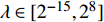
1) Parameter Determination for MLSSVM-based Model Using the Standard Data: The purpose of optimization considered here is to find a MLSSVM regression model with satisfactory generalization. In this experiment, the energy efficiency dataset [36] is employed which is downloaded from UCI machine learning repository. 500 data points are selected to train this model and 200 data points are used as testing data. The MLSSVM model has three parameters to be configured and the energy efficiency dataset contains two output responses. Then, the optimization problem with three decision variables and two objective variables is considered according to (25) and (26).

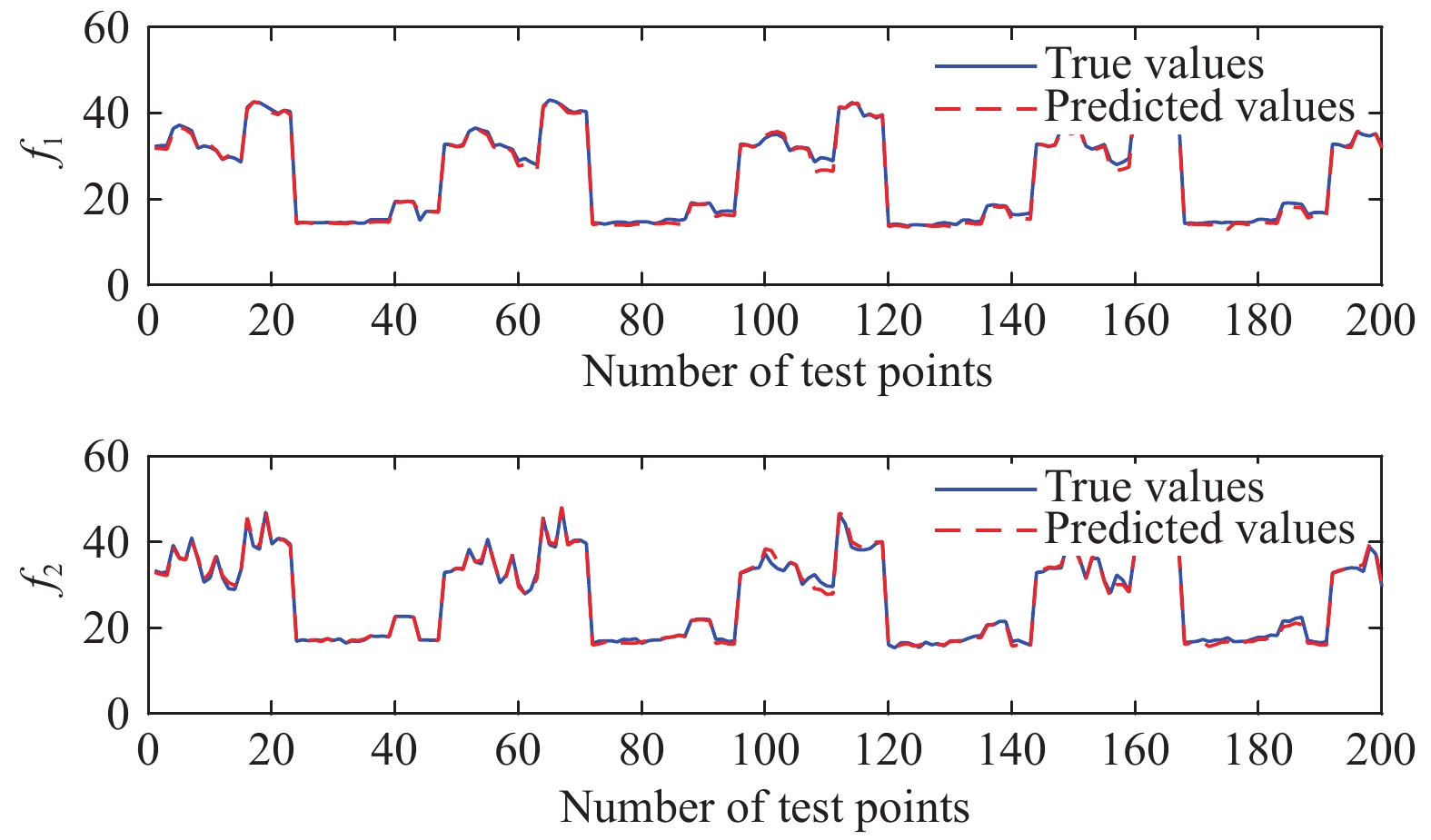
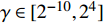
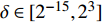
The optimal parameter configuration corresponds to the minimum of the mean square error between the predicted and real values. The $i\mathrm{th}$ parameter configuration is expressed as $MSE({\theta}_{i}) = MSE_{1}({\theta}_{i})+MSE_{2}({\theta}_{i})$, where $MSE_{1}({\theta}_{i})$ indicates the mean square error between the predicted values and the real values for the objective 1 and $MSE_{2}({\theta}_{i})$ represents the mean square error between the predicted values and the real values for objective 2. $\min(MSE({\theta}_{i}))$ corresponds to the MLSSVM model with the best prediction performance. Since the order of magnitude of the mean square error is different, $MSE_{1}({\theta}_{i})$ and $MSE_{2}({\theta}_{i})$ need to be normalized. In this experiment, 10 independent experiments are conducted and the maximum number of the fitness evaluations is set to 300 and 500. The statistical results of the experiment are shown in Table II, where MSE1, MSE2 and MSE represent the mean (the corresponding standard deviation) of $MSE_{1}({\theta}_{i})$, $MSE_{2}({\theta}_{i})$ and $MSE({\theta}_{i})$, $i = 1, 2, \dots, 10$. The parameter setting of the PAL-SAPSO is the same as that in the experiments on benchmark problems. For the MLSSVM model, the parameter ranges are set to $\lambda\in [2^{-15}, 2^{8}]$, $\gamma\in [2^{-10}, 2^{4}]$ and $\delta\in [2^{-15}, 2^{3}]$.

Table  II.  Statistic Results for Parameter Determination of MLSSVM-based Model

	300 fitness evaluations				500 fitness evaluations
	MSE1	MSE2	MSE		MSE1	MSE2	MSE
MOPSO	9.15×10−1 (3.19×10−1)	6.97×10−1 (4.06×10−2)	1.61×10−1 (3.43×10−1)		8.63×10−1 (2.30×10−1)	6.89×10−1 (2.97×10−2)	1.55×10−1 (2.43×10−2)
dMOPSO	7.92×10−1 (1.10×10−1)	7.22×10−1 (1.43×10−1)	1.51×10−1 (1.36×10−1)		8.25×10−1 (1.15×10−1)	6.82×10−1 (2.28×10−2)	1.50×10−1 (1.06×10−1)
SMPSO	8.90×10−1 (2.53×10−1)	6.92×10−1 (4.53×10−2)	1.58×10−1 (2.65×10−1)		7.35×10−1 (1.45×10−1)	6.81×10−1 (3.24×10−2)	1.42×10−1 (1.52×10−1)
ALMOPSO	6.77×10−1 (5.98×10−2)	6.92×10−1 (4.53×10−2)	1.37×10−1 (6.93×10−2)		6.63×10−1 (9.20×10−2)	6.87×10−1 (1.59×10−2)	1.34×10−1 (8.12×10−2)

 | Show Table

DownLoad: CSV

With respect to the results obtained with the 300 fitness evaluations in Table II, it can be clearly seen that the values of MSE1 obtained by PAL-SAPSO are the smallest for objective 1; the values of MSE2 obtained by PAL-SAPSO are similar to the ones obtained by MOPSO and SMPSO for objective 2; the values of MSE obtained by PAL-SAPSO are the smallest. These facts indicate that the convergence and the stability of PAL-SAPSO are better than MOPSO, dMOPSO and SMPSO, and the performance of MLSSVM model obtained by PAL-SAPSO is the best. As for the results obtained with the 500 fitness evaluations, it can be seen that MOPSO, dMOPSO and SMPSO can effectively reduce the mean square error by increasing the number of fitness evaluations. A similar parameter configuration scheme is obtained by PAL-SAPSO with the 300 and 500 fitness evaluations. It appears that PAL-SAPSO can find the reasonable parameter configuration more effectively with the same number of fitness evaluations compared with MOPSO, dMOPSO and SMPSO. In order to illustrate the effectiveness of PAL-SAPSO more intuitively, the predicted results with the best parameter configuration scheme are shown in Fig. 3.

Figure  3.  The predicted results with MLSSVM.

DownLoad: Full-Size Img PowerPoint

2) Parameter Determination for MLSSVM Model Using Industrial Data: In this experiment, the goal of optimization is to accurately predict real variation for the gas holder level with the MLSSVM model. The blast furnace gas (BFG) system [37] consists of BFG converters for gas generation, pipeline networks for gas transportation, gas users for consumption and gas holder for temporary storage. As the only storage equipment and buffer unit of the pipe network, the gas holder level reflects the balance state of the generation and consumption of the gas in the pipe network. In order to simplify the problem, the inner relationships between the gas generation users and the gas consumption users are not considered. Then, the total gas generation flow, the total gas consumption flow, the 1# gas holder level at the first moment and the 2# gas holder level at the first moment are considered as the inputs. The 1# gas holder level and the 2# gas holder level are seen as the outputs. Based on samples from the input and output above, the MLSSVM model has three parameters need to be determined. Therefore, the optimization problem with three decision variables and two objective variables is considered according to (25) and (26).

To establish the MLSSVM model, the gas flow data over 4 weeks are randomly selected. The sampling interval of the time series data is one minute. The number of the training samples is set to 5040 (two weeks data). The process of predicting is triggered every 5 points (5 minutes) to predict the future 30-min gas flow. It takes about 127.50 s to carry out an exact fitness function evaluation (10-fold cross-validation). In order to achieve the optimization of the MLSSVM model within 12 hours, the maximum number of fitness evaluations is set to 300. Furthermore, in order to predict the real variation of the gas holder level, the dynamic optimization of the MLSSVM model (DMLSSVM) is carried out every 12 hours. The training samples of the DMLSSVM model are updated every 12 hours. For verifying the feasibility of the DMLSSVM model, a static MLSSVM model (SMLSSVM) is developed. The training samples of the SMLSSVM model are from the gas flow data of the first two weeks. The parameter setting of the PAL-SAPSO is the same as that in the experiments on benchmark problems. The parameter ranges of the MLSSVM model are set to $\lambda\in [2^{-15}, 2^{8}]$, $\gamma\in [2^{-10}, 2^{4}]$ and $\delta\in [2^{-15}, 2^{3}]$

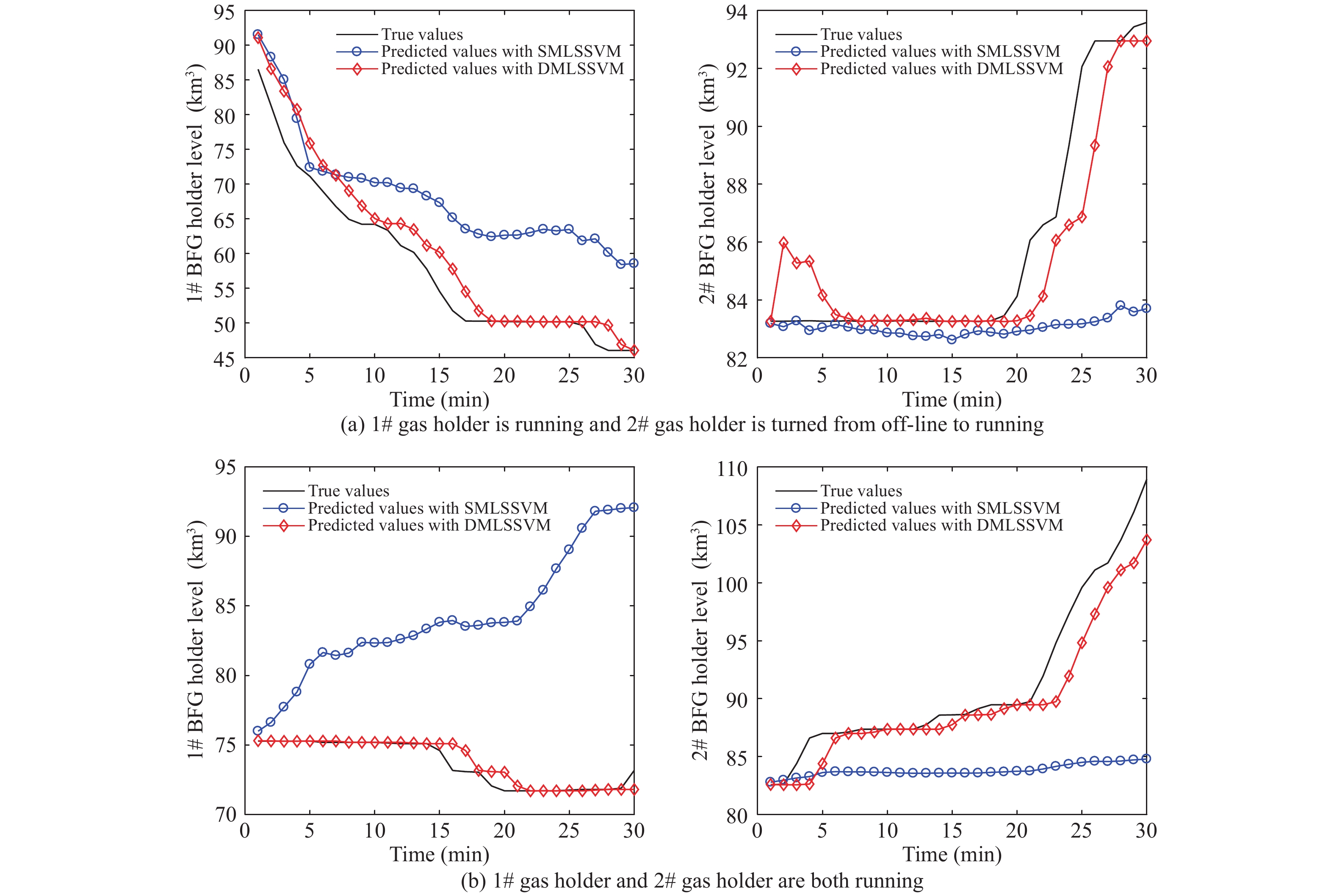
For verifying the effectiveness of PAL-SAPSO in the optimization problem on MLSSVM model driven by the gas flow data, two types of working conditions are selected as the representatives in this study: 1) 1# gas holder is running, 2# gas holder is turned from off-line to running; 2) 1# gas holder and 2# gas holder are both running. The corresponding simulation results are shown in Fig. 4 respectively. As shown in Fig. 4, DMLSSVM can effectively predict the change trend of 1# gas holder level and 2# gas holder level for two types of working conditions. Although it roughly predicts the changing trend of 1# gas holder level in the first type of working conditions, SMLSSVM fails to estimate the tendency of 2# gas holder level and the 1# and 2# gas holder level in the last type of working condition. In all, based on the dynamic optimization with PAL-SAPSO, the real changing trend of the gas holder level can be accurately forecasted with the parameter optimized MLSSVM model.

Figure  4.  The simulation results obtained by algorithms on two types of working condition.

DownLoad: Full-Size Img PowerPoint

V. Conclusion

In this paper, a surrogate-assisted PSO with Pareto active learning is proposed to solve the multi-objective optimization problem with high computational cost. In this algorithm, PSO is regarded as a sampler to generate candidate solutions. The performance of the PSO optimizer is improved by pre-selecting results from the candidate solutions with the improved $\varepsilon$-PAL. To improve the performance of the sampler, a hybrid mutation sampling method based on simulated evolution is proposed, which takes into account fast convergence and the diversity of distribution. In addition, a new method for determining the parameter ε is suggested where the number of the active sampling is used as an evaluation index of classification cost. The effectiveness of the proposed algorithm is verified by eight standard test problems. Compared with MOPSO, dMOPSO and SMPSO, the experimental results demonstrated that the Pareto optimal solutions obtained by the proposed algorithm has better convergence and distribution. In addition, comparative studies are also conducted on two MLSSVM model optimization problems, in which the advantage of determining effective parameter configuration schemes for the proposed method is verified on not only the standard data but also the real-world applications.

A few parameters (e.g., the value of the classification cost $T$) in the proposed algorithm must be predefined by the user, which do affect the performance of algorithms and must be defined properly. Therefore, more attention will be paid to address this issue. In addition, the performance of the proposed algorithm on expensive optimization problems with high dimension also remains to be verified.