Adaptive Fuzzy Dynamic Surface Control of Flexible-Joint Robot Systems With Input Saturation

Ⅰ. INTRODUCTION

In recent years, considerable attention has been paid in tracking control of flexible-joint (FJ) robot systems with robot dynamics and actuator dynamics. A number of different control strategies have been reported for FJ robot tracking control; Chang et al. [1] provided an excellent review of these methods including feedback linearisation control [2], passivity control [3], singular perturbation control [4], adaptive sliding mode control [5], proportional-derivative control [6], observer-based control [2] and adaptive backstepping control [7]-[9]. The backstepping technique is one of the popular techniques to control nonlinear systems with parameter uncertainty during the past two decades. However, the backstepping technique has a drawback called "explosion of complexity". To solve the problem, Swaroop et al. [10] proposed an adaptive dynamic surface control (DSC) technique to first solve the problem by introducing a first-order filter at each step of the traditional backstepping design. Many other important research results combined with DSC have also been presented. For example, the authors in [11] considered the problem of a class of strict-feedback nonlinear systems with input saturation using adaptive neural dynamic surface control. Su [12] proposed an output-feedback tracking controller for a class of nonlinear non-minimum phase systems.

Neural networks or fuzzy logic systems (FLSs) have been often used to approximate unknown continuous functions because of their universal approximation properties [13]. Since Polycarpou [14] first developed a neural-based adaptive controller for a class of nonlinear systems and Wang et al. [15] first presented a class of fuzzy systems to approximate a controller for a nonlinear ball and beam system, adaptive neural control and fuzzy control of nonlinear systems have received extensive attention in theoretical and practical applications [16]-[28]. It is worth mentioning that some of these articles have improved the structure of neural networks or fuzzy systems by combining network techniques. The successful application of these technologies will greatly enhance the control of nonlinear systems in the future. On the other hand, many researchers have used fuzzy systems to address control design of nonlinear systems in recent years. For instance, an adaptive fuzzy output feedback control method for single-input-single-output (SISO) nonlinear systems are presented to solve the problems associated with unmodeled dynamics and dynamic disturbances [18]. The FLSs are extended to control FJ robots [19], and an adaptive type-2 fuzzy logic controller (FLC) is proposed for FJ robotic manipulators with dynamical uncertainties [20].

As it is well known, input saturation may lead to control failure due to limited input amplitude of the actuator. Significant research efforts have been made to solve input saturation in the past few years [29]-[35]. The authors ([30] and [31]) solved the problem of uncertain systems with input saturation using fuzzy output control, and the problem of saturation is solved by approximation with a smooth function. Combining fuzzy logic systems and a small-gain approach, Zhou et al. [32] considered the problem of input saturation for single-input and single-output nonlinear systems with the nonstrict-feedback form. To solve the input saturation issue in MIMO nonlinear time-delay systems, a fuzzy sliding-mode control is presented [33]. While all of the above studies have made progress and achieved good results, the problem of an "explosion of complexity" needs to be further investigated. Moreover, the tracking control of FJ robot systems with input saturation also needs to be taken into account in practice.

Inspired by the above research, we present an adaptive fuzzy tracking control system for single-link FJ robots by combining the backstepping technique with DSC design. In order to solve the issue of input saturation that is nonsmooth in the system, we choose a smooth function to approximate it such that the backstepping technique can be utilized to design the controller. FLSs are applied to approximate unknown continuous functions. Adaptive DSC design is used to overcome the problem of the "explosion of complexity" by introducing auxiliary first-order filters. Lyapunov stability analysis shows that the uniform boundedness of all signals within the closed-loop system is guaranteed. The main contributions of this paper could be summarized in two parts:

1) An adaptive fuzzy DSC control strategy is presented for single-link flexible-joint robot systems with input saturation;

2) Only one adaptive law is designed by estimating the maximum value of the square of the weight vector norm. In this way, the structure of the designed controller is simple and the computational burden is significantly reduced.

It is shown that the proposed control scheme can guarantee the semi-global uniform ultimate boundedness of all signals in the closed-loop system. A comparison is conducted to show that the improved DSC method can reduce the computational burden by almost two thirds in comparison with the standard DSC method.

The remainder of this paper is organized as follows. Problem formulation and preliminaries are given in Section Ⅱ. Adaptive fuzzy control design using DSC and stability analysis is presented in Section Ⅲ. Section Ⅳ provides simulation results to show the effectiveness of the proposed scheme. The conclusions are included in Section Ⅴ.

Ⅱ. PROBLEM FORMULATION AND PRELIMINARIES

Throughout this paper, $\tilde{(\cdot)}=(\cdot)-\hat{(\cdot)}$, where $\hat{(\cdot)}$ is the estimate of $(\cdot)$, $(\cdot)^T$ denotes transposition of a vector, $\rVert \cdot\rVert$ denotes the two-norm.

According to the Euler-Lagrangian equations, the single-link FJ robot dynamics and actuator dynamics can be obtained as follows [5], [36]:

where $q$, $\dot{q}$, $\ddot{q}\in \mathbb{R}$ denote the link position, velocity, and acceleration, respectively. $M$, $g$, $L\in\, \mathbb{R}$ are the mass of the link, gravity acceleration, and the length of the link, respectively. $q_m$, $\dot{q}_m$, $\ddot{q}_m\, \in \mathbb{R}$ denote the rotor angular position, velocity, and acceleration, respectively. $K$, $J$, $B\in \mathbb{R}$ represent the coefficients of joint stiffness, the joint flexibility, and the natural damping, respectively, where $B$ is unknown. $F(\dot{q})\in \mathbb{R}$ represents friction. $u(v(t))$ denotes the characteristic of input saturation. $v(t)\in \mathbb{R}$ is the control input to be designed of the input saturation. $u(\cdot)$ denotes the plant input which is described by the following equation

where $u_M$ denotes the bound of the plant input $u(t)$. It can be observed that the plant input $u(t)$ is not smooth; as the result, the backstepping technique can not be utilized directly. In such a situation, we adopt a smooth function to approximate the saturation characteristic as below:

with $\rho(v)$ being the approximation error. Then, the $u(v(t))$ in (3) can be written as

Since the sat function in (3) and tanh function in (4) are both bounded functions, $\rho(v)$ in (5) is also a bounded function and its bound is

For the convenience of controller design, we utilize the mean-value theorem to tackle the function $g(v)$.

where $v^{\mu}=\mu v+(1-\mu)v^0$ with $0<\mu<1$.

By choosing $v^0=0$, one can obtain

By initializing $g(0)=0$ and using the above equation, we can have the following result

Letting $h(v)=\frac{\partial g(v)}{\partial v}\vert_{v=\mu v}$, the following equation satisfies

Since the tanh function and control input $v$ in (10) are both bounded, $h(v)$ in (10) is also a bounded function and its bound is

To facilitate design, the following assumptions are needed.

Assumption 1 [37]: The desired signal $y_d$ is continuous and available, and $[y_d, \dot{y}_d, \ddot{y}_d]^T\in\Omega_d$ with the known compact set $\Omega_d=\left\{[y_d, \dot{y}_d, \ddot{y}_d]^T:y^2_d+\dot{y}^2_d+\ddot{y}^2_d\le B_0\right\}\in \mathbb{R}^3$, where $B_0$ is a known positive constant.

Assumption 2: The minimum value of $h(v)$ in (11) is known. That is, the constant $h_m$ is known and we can use it in the process of design.

Remark 1: Since the control input $v$ we will design later is always bounded in the actual system, there exists a minimum value for $h(v)$ and Assumption 2 is reasonable in the actual system. On the other hand, the boundary value of control input $v$ can be obtained when the input saturation is not considered into. According to $h_m=1-\tanh^2(\frac{\bar{v}_{\max}}{u_M})$, the constant $h_m$ can be obtained in the simulation, where $\bar{v}_{\max}$ denotes the maximum value of $v$ in the absence of input saturation, and $u_M$ denotes the bound of the plant input $u(t)$. The detailed explanation about $h_m$ is illustrated in appendix.

Based on the above discussion and analysis, we transfer the system (1) and (2) with new state variables. Let $x_1=q, \ x_2=\dot{q}, \ x_3=q_m$ and $x_4=\dot{q}_m$. Then, the robot dynamics and actuator dynamics of (1) and (2) can be described as follows:

The control objective is to design an adaptive fuzzy controller $v$ for the single-link FJ robot system to guarantee that the system output $y$ can track the desired trajectory $y_d$, and all the signals in the closed-loop system are bounded.

In this paper, we will utilize FLSs to approximate the unknown function $f(x)$ and the results of approximation can be represented as

where $W^*=[w^*_1, \dots, w^*_N]^T$, $\Psi(x)=[\psi_1(x), \dots, \psi_N(x)]^T$.

Only one adaptive parameter needs to be updated in this paper, which reduces the computational burden significantly. The parameter $\theta$ is defined as

Lemma 1 [31]: For a continuous unknown function $f(x)$ defined on a compact set $\Omega$, there exists a fuzzy system $W^T\Psi(x)$ such that for any given constant $\varepsilon>0$, the following inequality holds

Ⅲ. ADAPTIVE FUZZY DSC DESIGN

In this section, we will attempt to design an adaptive DSC controller with FLSs for the single-link FJ system. The design of adaptive DSC is based on the following change of coordinates:

where $x_1, x_i, y_d, \omega_i\in \mathbb{R}, i=2, 3, 4$, $\omega_i$ is the output of the first-order filter with $\alpha_{i-1}$ as the input, and $\alpha_{i-1}$ is an intermediate control. The first-order filter with time design constant $\tau_i$ is defined as

with the filter errors

The recursive design procedure contains 4 steps. At each recursive step $i$, the FLSs may be used to approximate unknown system dynamics, and then the virtual control law $\alpha_i$ and the first-order filter are designed.

Step 1: Considering the first equation of system (12) using (16) and (18) gives

Choose a Lyapunov function candidate as

Subsequently, taking the time derivative of $V_{s_1}$ and using (19) yields

Next, construct the virtual control law $\alpha_1$ as

where $k_1$ is a positive design parameter. Substituting (22) into (21) yields

Using Young's inequality, the following inequalities hold

Then, substituting (24) and (25) into (23) produces

Let $\alpha_1$ pass through a first-order filter with the filter time design constant $\tau_2$ to introduce a new filter variable $\omega_2$ as

Based on $y_2=\omega_2-\alpha_1$, $\dot{\omega}_2=\frac{\alpha_1-\omega_2}{\tau_2}=-\frac{y_2}{\tau_2}$ is satisfied. And then the time derivative of $y_2$ can be obtained as

Define $\vert k_1\dot{s}_1-\ddot{y}_d\vert=\vert -\dot{\alpha}_1\vert\le\zeta_2(\dot{s}_1, \ddot{y}_d)$, where the continuous function $\zeta_2(\dot{s}_1, \ddot{y}_d)=\zeta_2(s_1, s_2, y_2, y_d, \dot{y}_d, \ddot{y}_d)$. Further, we have

For clarity of design, $\zeta_2(s_1, s_2, y_2, y_d, \dot{y}_d, \ddot{y}_d)$ is abbreviated as $\zeta_2$ in the following design. By combining (28) with (29) and using the Young's inequality, one has

Next, we construct the following Lyapunov function as

Combining (26) with (30), the time derivative of $V_1$ can be gained as

Step 2: The time derivative of $s_2$ is

In view of (16) and (18), (33) is rewritten as

Define

where $f_1$ denotes a unknown continuous function, which can be approximated by using FLSs later. Then, (34) can be rewritten as

Construct the following Lyapunov candidate function based on the virtual error and the adaptive parameter

where $\tilde{\theta}=\theta-\hat{\theta}$, $\hat{\theta}$ is the estimate of $\theta$ which is defined in (14) and $\gamma$ is a positive design constant. Taking the time derivative of $V_{s_2}$ yields

Substituting (36) into (38) produces

Next, a fuzzy system $W^T_1\Psi_1(X_1)$ is employed to approximate $f_1$ such that for any given constant $\varepsilon_1>0$, $f_1$ is written as

where $\delta_1(X_1)$ is the approximation error with $\varepsilon_1$ being the bound of $\delta_1(X_1)$. Combining (40) with (39) gives

Using the Young's inequality, the following inequalities hold

Substituting (42) and (43) into (41) yields

Now, a virtual control signal can be chosen as

where $\hat{\theta}$ is the estimate of $\theta$. The adaptive law will be designed in the last step. Combining (45) with (44) gives

By using the Young's inequality, we have

Combining (47) and (48) with (46) yields

Next, we let $\alpha_2$ pass through a first-order filter with the filter time design constant $\tau_3$ to introduce a new filter variable $\omega_3$ as

Based on $y_3=\omega_3-\alpha_2$, $\dot{\omega}_3=\frac{\alpha_2-\omega_3}{\tau_3}=-\frac{y_3}{\tau_3}$ is satisfied. And then the time derivative of $y_3$ can be obtained as

By following the similar process to step 1, we define $\vert -\dot{\alpha}_2\vert\le\zeta_3(s_1, s_2, s_3, y_2, y_3, \hat{\theta}, y_d, \dot{y}_d, \ddot{y}_d)$. Further, one has

Let $\zeta_3$ represent $\zeta_3(s_1, s_2, s_3, y_2, y_3, \hat{\theta}, y_d, \dot{y}_d, \ddot{y}_d)$ for clarity. Combining (51) with (52) and using Young's inequality yields

Next, we construct the following Lyapunov function as

Using (49) and (53), the time derivative of $V_2$ can be obtained as

Step 3: Combining (16) with (18), the time derivative of $s_3$ can be obtained as

Design the following Lyapunov candidate function as

By taking the time derivative of $V_{s_3}$, we get the following result

We then choose the virtual control law $\alpha_3$ as

where $k_3$ is a positive design parameter. Substituting (59) into (58) yields

Using Young's inequality, the following two inequalities hold

By substituting (61) and (62) into (60), we have

Next, let $\alpha_3$ pass through a first-order filter with the design constant $\tau_4$ to introduce a new filter variable $\omega_4$ as

Repeating steps similar to (50) and (51) yields

We define $\vert k_3\dot{s}_3-\ddot{\omega}_3\vert=\vert -\dot{\alpha}_3\vert\le\zeta_4(\bar{s}_4, \bar{y}_4, \hat{\theta}, y_d, \dot{y}_d, \ddot{y}_d)$, where $\bar{s}_4=[s_1, s_2, s_3, s_4]$, $\bar{y}_4=[y_2, y_3, y_4]$. Based on (65), one has

Simplify $\zeta_4(\bar{s}_4, \bar{y}_4, \hat{\theta}, y_d, \dot{y}_d, \ddot{y}_d)$ as $\zeta_4$ for the convenience of design. Combining (65) with (66) and using Young's inequality gives

Next, we construct the following Lyapunov function as

Combining (63) with (67), the time derivative of $V_3$ can be obtained as

Step 4: The time derivative of $s_4$ is

Choose a Lyapunov function as

Then, combining (70) with (71) and using the Young's inequality, the time derivative of $V_4$ can be obtained as

where $f_2=J^{-1}\Big(-Bx_4-K(x_3-x_1)\Big)-\dot{\omega}_4$ denotes a continuous function. Then, a fuzzy system $W^T_2\Psi_2(X_2)$ is employed to approximate $f_2$ such that for any given $\varepsilon_2>0$, $f_2$ is written as

where $\delta_2(X_2)$ is the approximation error with $\varepsilon_2$ being the bound of $\delta_2(X_2)$. Substituting (73) into (72), using Young's inequality, and repeating the steps similar to (42) and (43) yields

Now, we are ready to design the actual controller $v$ as

Remark 2: It is worth noting that we utilize FLSs to approximate the unknown continuous function $f_1$ and known continuous function $f_2$ in Step 2 and this step, respectively. It is better not to use fuzzy logic systems to estimate the known continuous function $f_2$ in this step because of the existence of approximation error. However, the impact of this processing on system performance is negligible for because FLSs can make very accurate approximations. The main reason for this is to make the design similar to that in Step 2 and to make the form of the controller simple.

Substituting (75) into (74) yields

In order to facilitate stability analysis, consider the following Lyapunov function as

With the help of (32), (55), (69) and (76), the time derivative of $V$ can be obtained as

where $\bar{k}_1=k_1-2$, $\bar{k}_2=k_2-\frac{K^2}{ML^2}-\frac{3}{4}$, $\bar{k}_3=k_3-2-\frac{1}{2ML^2}$, $\bar{k}_4=k_4-\frac{5}{4}$, $\bar{\tau}_2=\frac{1}{\tau_2}-\frac{5}{4}$, $\bar{\tau}_3=\frac{1}{\tau_3}-1-\frac{1}{2ML^2}$, $\bar{\tau}_4=\frac{1}{\tau_4}-\frac{5}{4}$.

For any $B_0>0$ and $p>0$, the sets $\Omega_d=\{(y_d, \dot{y}_d, \ddot{y}_d):y^2_d+\dot{y}^2_d+\ddot{y}^2_d\le B_0\}$ and $\Omega_i=\{[\bar{s}^T_i, \bar{y}^T_i, \hat{\theta}]^T:\sum^i_{j=1}V_j\le p\}, i=1, 2, 3, 4$ are compact in $\mathbb{R}^3$ and $\mathbb{R}^{2i}$, respectively. Therefore, $\zeta_j$ has a maximum $T_j$ on $\Omega_j\times\Omega_i$, $j=2, 3, 4$.

Subsequently, design the following adaptation law as

Now, the fuzzy DSC design procedure is complete. The main results are summarized as follows.

Theorem 1: Consider the closed-loop flexible-joint robot system consisting of (1) and (2) with Assumptions 1 and 2, the virtual control signals (22), (45), and (59), the actual controller (75), and the adaptive law (79); Moreover, assume that the unknown continuous function $f_1$ and $f_2$ can be approximated by FLSs when the approximation errors are bounded. For any given bounded initial conditions, all the signals in the closed-loop system are bounded, and the output of the system can track the desired trajectory with the tracking error converging to a small domain around the origin.

Proof: By using the relationship of $\hat{\theta}=\theta-\tilde{\theta}$ and Young's inequality, one has

Substituting (79) into (78) and using (80), the following design parameters are chosen to guarantee that (78) is stable:

Then, by substituting (81) into (78) and using (80), one can obtain the following result:

where $\alpha_0$ is a positive design parameter, and $C$ is a bounded constant which is defined as

Remark 3: The choice of design parameters follows the principles of the subsystem. For example, for the design of parameter $k_1$, equation (82) is the final form we expect. By combining equation (77) with (78), we have $-\bar{k}_1s^2_1\le -\alpha_0\frac{s^2_1}{2}$, and eventually we can obtain $k_1\ge 2+\frac{\alpha_0}{2}$. The other design parameters are the same as this. During the simulation process, we found that the design parameter $k_2$ has greatest influence on system performance and better performance can be obtained by selecting larger $k_2$. Furthermore, design parameters $\tau_i~(i=2, 3, 4)$ need to be carefully chosen. If the selected parameter $\tau_i$ is too large, it will cause the designed controller to oscillate. Conversely, if the selected parameter $\tau_i$ is too small, it will result in a large controller output. Other design parameters such as $a_1, a_2, h_m$ also need to be adjusted accordingly.

Let $\alpha_0>C/p$, where a detailed description of $p$ is made following (78). Then $\dot{V}\le0$ on $V=p$. That is, $V\le p$ is a invariant set, i.e., if $V(0)\le p$, then $V(t)\le p$, for all $t\ge0$. By solving the inequality of (82), we can obtain

which means that

Therefore, all signals in the closed-loop system, i.e., $s_i, y_j, \tilde{\theta}$ $(i=1, 2, 3, 4, j=2, 3, 4)$ are semi-globally uniformly ultimately bounded. Since $x_1=s_1+y_d$, $x_1$ is also bounded from the boundedness of $s_1$ and $y_d$. The boundedness of $x_2$ follows from boundedness of $\alpha_1(\dot{y}_d, s_1)$ and the fact that $x_2=s_2+y_2+\alpha_1$. Similarly, the boundedness of $x_3$ and $x_4$ can be obtained. The boundedness of $\hat{\theta}$ can be ensured from the boundedness of $\tilde{\theta}$ and $\theta$. From (75), because $v$ is a function of $s_4$, $\hat{\theta}$ and $\Psi_2(X_2)$, which are all bounded, $v$ is also bounded. Moreover, by appropriately choosing the design parameters, such as increasing $\gamma$ or decreasing $a_1 , a_2$, we ensure that the tracking error converges to a small neighborhood around 0 such that the output of the system can track the desired trajectory very well.

Ⅳ. SIMULATION RESULTS

To illustrate the effectiveness of the proposed approach, consider the following dynamics of the single-link FJ robot system:

The friction term is selected as $F(\dot{q})=B_1\cos\dot{q}$. Table Ⅰ gives the system parameters and the desired reference trajectory is given as $y_d=0.5\big(\sin(t)+\sin(0.5t)\big)$.

Table  Ⅰ.  PARAMETERS OF THE SINGLE-LINK FJ ROBOT SYSTEM

Parameters	Description	Values	Unit
$M$	the mass of link	0.25	kg
$L$	the length of link	1	m
$g$	gravity acceleration	9.8	$\text{m}/\text{s}^2$
$K$	joint stiffness	2	N$\cdot \text{m}/\text{rad}$
$B$	damping coefficient	0.6	none
$B_1$	friction coefficient	0.01	none
$J$	joint flexibility	0.001	$\text{m}/\text{s}^2$

 | Show Table

DownLoad: CSV

For the FLSs, the number of the fuzzy rules $N$ is selected as $N=7$ and the Gaussian function $\psi_i(x)$ is chosen as $\psi_i(x)=\exp[-(x-\mu_i)^T(x-\mu_i)/(\eta^2_i)]$, where the center vector $\mu_i=[-3\ -2\ -1\ 0\ 1\ 2\ 3]$ and the width of the Gaussian function $\eta_i=1, i=1, 2, \ldots, N$.

We choose design parameters as $\alpha_0=\gamma=0.5$, $h_m=0.03$, $\tau_2=\tau_3=\tau_4=0.002$, $k_1=2.3$, $k_2=17$, $k_3=k_4=6$, $a_1=0.01$, $a_2=25$, initial state values $q=0.1$, $\dot{q}=0.2$, $q_m=0.5$, $\dot{q}_m=0.5$, the initial values of the first-order filters are $\omega_2=\omega_3=\omega_4=0.5$, the boundary of the plant input is selected as $u_M=2$ and the initial value of the square for the weight vector norm is chosen as $\theta=5$.

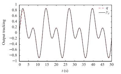
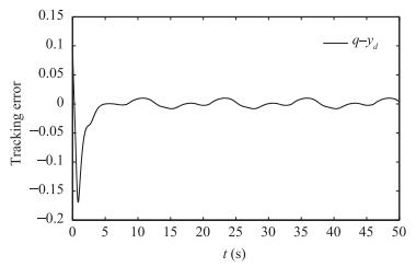
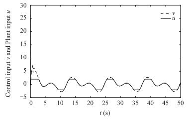
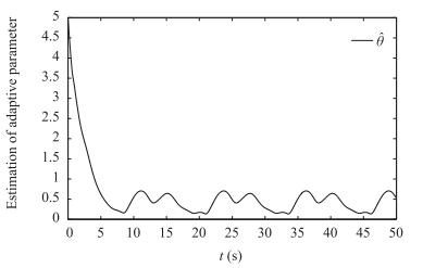
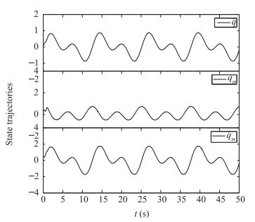
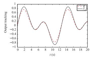
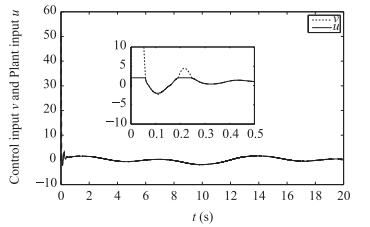
The results of the simulation are shown in Figs. 1-5. It can be seen from Figs. 1 and 2 that the system output $q$ can track the desired trajectory $y_d$ well. Fig. 3 shows the control input $v$ and plant input $u$, respectively. We can observe that the plant input $u$ satisfies $\vert u\vert\le u_M$, which indicates the effectiveness of our proposed approach. The response curve of adaptive parameter is illustrated in Fig. 4. Fig. 5 shows that the state signals are bounded.

Figure  1.  Trajectories of the link position $q$ and the desired trajectory $y_d$.

DownLoad: Full-Size Img PowerPoint

Figure  2.  Tracking error for the single-link robot.

DownLoad: Full-Size Img PowerPoint

Figure  3.  Control input v and plant input u of the single-link robot.

DownLoad: Full-Size Img PowerPoint

Figure  4.  Estimation of the maximum value of the square for the vector norm of the weight.

DownLoad: Full-Size Img PowerPoint

Figure  5.  Trajectories of link velocity $\dot{q}$, rotor angular position $q_m$ and rotor angular velocity $\dot{q}_m$

DownLoad: Full-Size Img PowerPoint

To further demonstrate the main contribution of our proposed control scheme, we apply the standard DSC method [37] which updates the weight vector to the same single-link FJ robot system in (86).

Similar to the design procedure in Section Ⅲ, in order to save space, we only give the final design results. The virtual controller and actual controller are chosen as

and the adaptive law is designed as

For fairness of comparison, we use the same system parameters and the same initial conditions in simulation. FLSs and the desired reference signal are the same as before. Design parameters are chosen as $\Gamma_1=\Gamma_2=\text{diag}(0.5, 0.5, 0.5, 0.5, 0.5, 0.5, 0.5), \sigma_1=\sigma_2=0.1, k_1=2.5, k_2=5, k_3=2.5, k_4=3,$ and $\tau_2=\tau_3=\tau_4=0.02$. Other design parameters are consistent with the above design parameters. The initial values of the weight vector are chosen as $W_1=W_2=[0.5;0.5;0.5;0.5;0.5;0.5;0.5]$.

The results of the simulation using standard DSC which updates the weight vector are shown in Figs. 6 and 7. Considering the running time of the program, the simulation time is set to 20 s since long simulation time will consume more time than the improved DSC scheme. Trajectories of the link position $q$ and the desired trajectory $y_d$ using the standard DSC method are shown in Figs. 6 and 7, which illustrate the control input $v$ and plant input $u$ of the single-link robot. It is obvious that the control performance of our proposed improved DSC scheme is better than the standard DSC method comparing Figs. 1-3 with Figs. 6 and 7.

Figure  6.  Trajectories of the link position $q$ and the desired trajectory $y_d$ by using standard DSC method.

DownLoad: Full-Size Img PowerPoint

Figure  7.  Control input $v$ and plant input $u$ of the single-link robot by using standard DSC method.

DownLoad: Full-Size Img PowerPoint

Remark 4: It should be noted that the objective of comparison experiments is to illustrate the fact that only one adaptation parameter can reduce the computational burden significantly. The time complexity of the two control schemes rather than the control performance is the main concern here.

The solving time and total running time of the improved DSC scheme, which updates the maximum value of weight vector norm, and standard DSC method, which updates the weight vector, are shown in Table Ⅱ and Table Ⅲ.

Table  Ⅱ.  STANDARD DSC TIME CONSUMING VS. IMPROVED DSC TIME CONSUMING: SOLVING TIME (UNIT: S)

Simulation time	Improved DSC	Standard DSC
50	10.7	29
40	8.6	22.6
30	6.5	16.9
20	4.5	11.5
10	2.2	5.8
5	1.1	2.9

 | Show Table

DownLoad: CSV

Table  Ⅲ.  IMPROVED DSC TIME CONSUMING VS. STANDARD DSC TIME CONSUMING: TOTAL RUNNING TIME (UNIT: S)

Simulation time	Improved DSC	Standard DSC
50	11	$\backslash$
40	8.7	$\backslash$
30	6.7	$\backslash$
20	4.5	452
10	2.3	107
5	1.2	26

 | Show Table

DownLoad: CSV

Remark 5: The solving time and total running time are obtained under the condition that the program is run three times and averaged. The program runs on MATLAB R2014a, which is installed on a Win 10 OS equipped with 4 GB RAM and an Intel Core i5-6300HQ processor. The solving time refers to the time it takes for the algorithm to solve the problem, which represents the computational complexity of the algorithm. Total running time includes solving time and subsequent processing time. In fact, we expect to shorten the solving time to reduce the computational burden, and we prefer to reduce the total running time to quickly select design parameters to optimize control performance.

It can be observed from Table Ⅱ that the improved DSC method is almost three times faster than the standard DSC method in terms of simulation time. We can see that the total running time of the improved DSC method is much less than standard DSC method from Table Ⅲ. With the increase of simulation time, the time consumed also increases exponentially for the standard DSC method. Moreover, the advantage of the improved method is more obvious as system order and fuzzy rules increase. From the results of the comparison study, it can be concluded that the proposed scheme using only one adaptive parameter can reduce the computational burden significantly.

Ⅴ. CONCLUSION

This paper considers the tracking control problem of single-link flexible-joint robot system with input saturation using an adaptive fuzzy DSC, where the saturation problem is solved by a smooth function with the help of the mean-value theorem. The problem of an "explosion of complexity" is overcome by the adaptive DSC. The developed adaptive fuzzy control scheme can guarantee that all signals in the closed-loop system are uniformly ultimately bounded. The simulations on a single-link robot system show that the system output tracks the desired trajectory well under the input saturation. Comparison studies show that the proposed scheme can reduce the computational burden by nearly two-thirds in comparison with the standard method.

It should be pointed out, however, that our proposed DSC scheme does not consider the errors caused by the introduction of filters, which may limit performance of the system. Future research may investigate this potential problem associated with the DSC approach.

APPENDIX. SUPPLEMENTARY EXPLANATION OF CONSTANT $h_m$

In (10), $h(v)$ is defined as

and

Next, we will discuss how to select the minimum value $h_m$ of $h(v)$ in simulation. The following two cases should be considered.

Case 1: When $v>0$, there are still two cases should be considered. That is, when $0<v\le u_M$, $h_m$ can be determined as

where $h_{m1}=0.42$. When $v>u_M$, $h_m$ can be determined as

where $v^+_{\max}$ denotes the maximum value of input $v$ under the condition that $v$ is greater than zero in the simulation. In the actual controller, the input $v$ is always bounded. Therefore, we can choose a bigger $v_{\max}$ to determine $h_{m2}$.

Case 2: When $v<0$, the results are similar to case 1. That is, when $0<v\le u_M$, $h_m$ can be determined as $h_{m1}$. When $v>u_M$, $h_m$ can be determined as

where $\vert v^-\vert_{\max}$ denotes the maximum value of input $v$ in the case of $v$ less than zero in the simulation.

It should be noted that the input $v$ we discussed is carried out without input saturation. By combining with those two cases, we finally obtain