

Figure
1.
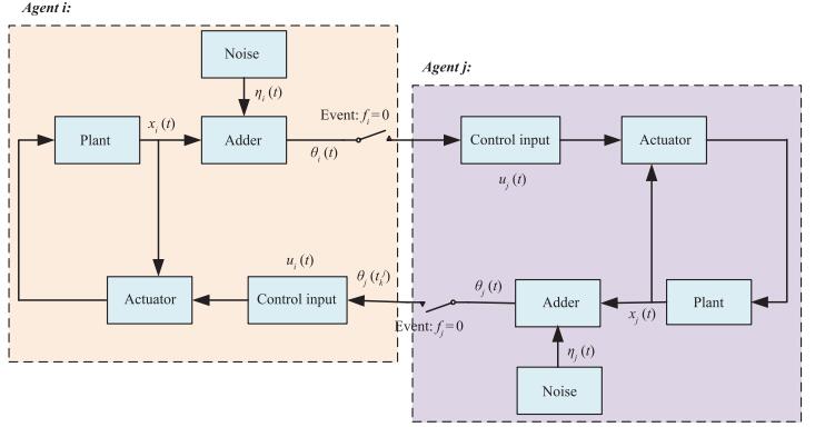
The event-triggered DPCA schematic architecture.
 Volume 6
Issue 1
Volume 6
Issue 1
IEEE/CAA Journal of Automatica Sinica
| Citation: | Aijuan Wang, Xiaofeng Liao and Haibo He, "Event-Triggered Differentially Private Average Consensus for Multi-agent Network," IEEE/CAA J. Autom. Sinica, vol. 6, no. 1, pp. 75-83, Jan. 2019. doi: 10.1109/JAS.2019.1911327

|
Mnetwork systems (MANSs) have been one of the focal points from many researchers due to its extensively real applications in a variety of scopes, such as biological systems, robotic teams, sensor networks, unmanned air vehicles formations, just to name a few [1]-[7]. Particularly, consensus problem, as a basic building block of MANSs' collective behaviors, has been widely investigated [8]-[14]. Moreover, a survey about theory and applications of consensus problems for MANSs is presented in [15]. The consensus of MANSs is that the states of all agents reach a common value by exchanging information among agents [16]-[22].
Recently, there is an increasing interest that is to apply the notion of privacy preserving into the consensus behaviors of the dynamical network systems (DNSs) [23]. It means that the network agents may not want to expose their initial states in the process of consensus computation. For example, in social networks (SNs), a group of individuals execute a prescribed procedure to obtain the common opinion on a subject [24] in which individual, however, may not want to divulgate its own true views on the subject. Subsequently, a few literatures have successfully studied the preserving-privacy problem in the context of consensus of MANSs [25]-[27]. It means that the algorithm not only achieves the agents' consensus, but also preserves the privacy of each agent' initial state against the other all agents. For example, privacy-preserving average consensus algorithms for MANSs are developed in [25] and [26]. The former just gives the condition that the initial state of one agent can be exactly recognized by the other agents. This motivates the latter to provide a quantitative condition that the initial state can be estimated perfectly. To extend the research of this filed, Duan et al. [27] propose a new privacy-preserving scheme and apply it to the maximum consensus algorithm for MANSs. The probability that the maximum state owner's identity is recognized by its neighbors is calculated. Later, differentially private, as an existing preserving-privacy approach, has gained remarkable attention due to its rigorous formulation and proven security properties, including resilience to post-processing and side information, and independence from the model of the adversary. Recently, there are a large number of results concerning the differentially private consensus problem for MANSs [28]-[31]. Huang et al. [28] firstly investigate the differentially private problem in the context of consensus of MANSs. Differentially private maximum consensus algorithm which achieves ϵ-differentially private for initial states of all agents and makes all agents converge to the maximum initial state value is developed [29]. For the common average consensus of MANSs, Nozari et al. [30] show that any differentially private algorithm cannot achieve exact average consensus. Following it, the authors in [30] systematically analyze the differentially private average consensus problem of MANSs in expectation [31]. This observation motivates us to develop different types of differentially private consensus algorithms (DPCAs) to preserve the initial states of the MANSs as well as achieve consensus for all agents' states.
It is worth noting that, on the other hand, the privacy-preserving consensus algorithms in [28]-[31] are continuous communication between agents and their neighbors. Continuous communication results in the waste of network resources and possibility blocks channels due to the mass of transmission data, which drives us to employ the intermittent communication techniques (ICTs). The event-triggered control (ETC) strategy, as a classical ICT, has successfully been applied to consensus control problem of the different kinds of MANSs for dramatically reducing communication among agents [32]-[43]. Model-based ETC is used for MANSs with quantization and time-varying delays [32]. Moreover, the ETC is proved to be an effective approach for the cooperative control problem of the nonlinear MANSs with unknown external disturbance [36], [37]. Based on the point, the latest article [44] firstly adopts the event-triggered scheme to the algorithm in [31]. To the best of authors' knowledge, there are few work to employ the ETC strategy in DPCA except for [44]. This observation inspires us to develop the corresponding ETC in some new DPCAs for reducing the communication among agents.
Motivated by the existing research in the above literature, in this paper, we develop a new event-triggered update law for all agents in MANSs as our differentially private consensus algorithm. The primary advantage of our proposed algorithm is that the mean square consensus of all agents in MANSs and the preservation of the privacy of each agent can be guaranteed simultaneously. In detail, the main contributions of our work are threefold: 1) A new distributed event-triggered DPCA is established for MANSs by introducing ETC strategy, which dramatically reduces the mutual communications among the agents. 2) Based on our algorithm, we carry out the detailed theoretical analysis, including its consensus, accuracy and differential privacy. Meanwhile, the sufficient condition of consensus, and its accuracy are derived, respectively. 3) An optimization problem is established to minimize the variance of the agents' convergence point according to the tradeoff between privacy level and algorithm's performance. It is found that the optimal value of the variance can be derived for the given privacy level.
The remainder of this paper is structured as follows. Section Ⅱ introduces the preliminaries for graph theory and probability theory, present the DPCA. The main results are established in Section Ⅲ, including three parts. First, the convergence analysis of the DPCA is presented. Second, the accuracy and differential privacy of the DPCA are guaranteed. Third, the optimization problem to minimize the variance of the agents' convergence point is established. Section Ⅳ provides some numerical examples to testify the validity of our results. Section Ⅴ contains some main conclusions and further research.
We consider a network of N agents interacting over a network topology modeled as an undirected and connected communication graph g=(V,ε,A). V={1,2,…,N} is a set of vertices and ε⊆V×V is a set of communication edge. (i,j)∈ε means that there is an edge between j and i. The neighbor set of agent i is defined as Ni={j∈V|(i,j)∈ε}. Note that i∈Ni, which means that there exists a self-loop for agent i. The cardinality of Ni for agent i is |Ni|. A=(aij)N×N is the connection weighted matrix of the graph g. The degree of agent i is defined as di=∑j∈Niaij and the Laplacian of the weighted digraph g is defined as L=D−A with D=diag{d1,d2,…,dN}. The graph g is connected if and only if for any two distinct agents i,j∈V, there is a path between j and i. Here, we order the eigenvalues of the matrix A in the decreasing order as λ1(A)≥λ2(A)≥⋯≥λN(A) and the eigenvalues of the Laplacian matrix L in the decreasing order as λ1(L)≥λ2(L)≥⋯≥λN(L)=0.
Consider the probability space (Ω,Σ,Pr, where, as usual, \Omega is the sample space, \Sigma is the collection of all events, and \Pr is the probability measure. A random variable is a measurable function X:\omega \in \Omega \to R, and we denote its expected value by E[X]. The variance of X is represented by {\mathop{\rm var}} \left( X \right) with {\mathop{\rm var}} \left( X \right) = E\left[ {{X^2}} \right] - E\left[ X \right]E\left[ X \right]. X \sim Lap\left( b \right) means that a zero mean random variable X obeys the Laplace distribution with its variance 2b^2. Its PDF is that f\left( {x;b} \right) = \frac{1}{{2b}}{e^{ - \frac{{\left| x \right|}}{b}}} for any x\in \mathbb{R}.
In this section, we develop a new update law of the discrete-time DPCA for each agent in MANSs as follows:
| \begin{align}\label{E1} &\; {\theta _i}\left( t \right) = {x_i}\left( t \right) + {\eta _i}\left( t \right)\nonumber\\ &\; {x_i}\left( {t + 1} \right) = {\alpha _i}{x_i}\left( t \right) + {\beta _i}\sum\nolimits_{j \in {N_i}} {{a_{ij}}{\theta _j}\left( t \right)} \end{align} | (1) |
where 0 < {\alpha _i}, {\beta _i} < 1 are the algorithm parameters, x_i(t) is the state of the agent i, \theta_i(t) is the state sending to its neighbors, and \eta_i(t) is the random noise, which obeys the Laplace distribution Lap\left( {{c_i}q_i^t} \right) with q_i\in (0, 1) and the positive constant c_i.
It is clearly seen that the communication among agents is continuous in the algorithm (1), which results in the waste of network resources. Motivated by this observation, the event-triggered DPCA is established as follows:
| \begin{align}\label{E2} &\;{\theta _i}\left( t \right) = {x_i}\left( t \right) + {\eta _i}\left( t \right)\nonumber\\ &\;{x_i}\left( {t + 1} \right) = {\alpha _i}{x_i}\left( t \right) + {\beta _i}\sum\nolimits_{j \in {N_i}} {{a_{ij}}{\theta _j}\left( {t_k^j} \right)} \end{align} | (2) |
where t_k^j is the event-triggered time instant for the agent j, and the next trigged time instant t_{k + 1}^i is determined by
| \begin{align}\label{E3} t_{k + 1}^i\!=\!\inf \!\left\{ {t:t\!>\!t_k^i, \left| {{e_i}\left( t \right)} \right|\!=\!{\sigma _i}\left| {\sum\nolimits_{j \in {N_i}} {\!\!\left({{\theta _j}\!\left( {t_k^j} \right)\!-\!{\theta _i}\left( {t_k^i} \right)}\!\! \right)} }\! \right|}\! \right\} \end{align} | (3) |
where {e_i}\left( t \right) is measure error with {e_i}\left( t \right) = {\theta _i}\left( {t_k^j} \right) - {\theta _i}\left( t \right), and 0 < {\sigma _i} < 1. The execution process of the algorithm (2) can be described as Fig. 1, where the control input u_i(t) is denoted by u_i(t)=\sum\nolimits_{j \in {N_i}} {{a_{ij}}{\theta _j}\left( {t_k^j} \right)}, i is a neighbor of agent j, and f_i(t) represents the event function with {f_i}\left( t \right) = \left| {{e_i}\left( t \right)} \right| - {\sigma _i}\left| {\sum\nolimits_{j \in {N_i}} {{\theta _j}\left( {t_k^j} \right) - {\theta _i}\left( {t_k^i} \right)} } \right|.
Remark 1: Our triggered condition (3) is more conservative. Admittedly, the triggered condition (3) is really not easy to satisfy due to the "=". But it is possible to satisfy if the size step is small enough. And, this similar form for event-triggered condition can be found in [45].
Remark 2: The proposed algorithm (1) is derived from the distributed algorithms (6)-(7) in [30], which is as follows:
| \begin{align}\label{E4} &\; {\theta _i}\left( t \right) = {x_i}\left( t \right) + {\eta _i}\left( t \right)\nonumber\\ &\;{y_i}\left( t \right) = \frac{1}{{\left| {N\left( i \right)} \right| + 1}}\sum\nolimits_{j \in {N_i} \cup \left\{ i \right\}} {{\theta _j}\left( t \right)}\nonumber\\ &\;{x_i}\left( {t + 1} \right) = \left( {1 - {\alpha _i}} \right){x_i}\left( t \right) + {\alpha _i}{y_i}\left( t \right). \end{align} | (4) |
However, the algorithm (4) can be viewed as a special case of our algorithm (1). It can be clearly seen that the parameters 0 < {\alpha _i}, {\beta _i} < 1 in our algorithm is more general than ones in [30]. On the other hand, the algorithm in [31] can be expressed as:
| \begin{align}\label{E5} &\;{\theta _i}\left( t \right) = {x_i}\left( t \right) + {\eta _i}\left( t \right)\nonumber\\ &\;{x_i}\left( {t + 1} \right) = {x_i}\left( t \right)\! +\! h\sum\nolimits_{j \in {N_i}} {{a_{ij}}\left( {{\theta _j}\left( t \right) - {\theta _i}\left( t \right)} \right)} \! +\! {s_i}{\eta _i}\left( t \right). \end{align} | (5) |
As the extension of the algorithm in [31], the latest article [44] adopts the event-triggered scheme to the algorithm (5), which forms the following:
| \begin{align}\label{E6} &\;{\theta _i}\left( t \right) = {x_i}\left( t \right) + {\eta _i}\left( t \right)\nonumber\\ &\;{x_i}\left( {t + 1} \right) = {x_i}\left( t \right) + h{u_i}\left( t \right) + {s_i}{\eta _i}\left( t \right)\nonumber\\ &\;{u_i}\left( t \right) = \sum\nolimits_{j \in {N_i}} {{a_{ij}}\left( {{\theta _j}\left( {t_k^j} \right) - {\theta _i}\left( {t_k^i} \right)} \right)}. \end{align} | (6) |
Note that without the term s_i\eta_i(t), the differentially privacy cannot be guaranteed, as is described in [31], [44]. Generally, for the general DPCA, the term s_i\eta_i(t) need not be included in the second equation. Actually, the term s_i\eta_i(t) have to be added to the algorithm (5) due to using the relative agents' information, which increases the computation load. Hence, the observation motivates us to use the absolute information such that the term s_i\eta_i(t) can be abandoned, which yields our algorithm (1).
Based on the above discussion, our algorithm (2) dramatically reduces the communication among agents by employing the ETC strategy, which is the main difference compared with algorithms in [30], [31]. And, the main differences from the [44] have three points: 1) Our algorithm uses the absolute information, which reduces the computation load between neighbors. 2) Our algorithm guarantees that every agent converges to the weighted average of initial states for all agents instead of the average of initial states in mean square. 3) In this paper, based on our algorithm, we further analyze the best achievable accuracy of our algorithm under the free parameters and the fixed privacy level.
In the following, some basic definitions and assumption are given.
Definition 1 (Convergence) [28]: The agents of MANSs are said to reach consensus in mean square if for any agents i, j = 1, 2, \ldots, N, \mathop {\lim }\limits_{t \to \infty } E{\left( {{x_i}\left( t \right) - {x_j}\left( t \right)} \right)^2} = 0 holds, where the expectation is over the coin-flips of the algorithm.
Definition 2 (Adjacency) [28]: Given \delta>0, the initial states of the two groups of network agents x_i^{\left( 2 \right)}\left( 0 \right), x_i^{\left( 1 \right)}\left( 0 \right) are \delta-adjacent, if there exists some i_0 such that
| \begin{align}\label{E7} \left| {x_{{i_0}}^{\left( 2 \right)}\left( 0 \right) - x_{{i_0}}^{\left( 1 \right)}\left( 0 \right)} \right| \le \left\{ \begin{array}{l} \delta {\kern 1pt} {\kern 1pt} {\kern 1pt} {\kern 1pt} {\kern 1pt} {\kern 1pt} {\kern 1pt} {\kern 1pt} {\kern 1pt} {\kern 1pt} {\kern 1pt} {\kern 1pt} {\kern 1pt} i = {i_0}, \\ 0{\kern 1pt} {\kern 1pt} {\kern 1pt} {\kern 1pt} {\kern 1pt} {\kern 1pt} {\kern 1pt} {\kern 1pt} {\kern 1pt} {\kern 1pt} {\kern 1pt} {\kern 1pt} {\kern 1pt} i \ne {i_0}. \end{array} \right. \end{align} | (7) |
Definition 3 (Differential Privacy) [28]: The algorithm (2) is \epsilon-differential privacy for any pair x_i^{\left( 2 \right)}\left( 0 \right) and x_i^{\left( 1 \right)}\left( 0 \right) of \delta-adjacent initial states, if
| \Pr \left[ {{\rm{Alg}}\left( {{x^{\left( 1 \right)}}} \right) \in \Xi } \right] \le {e^{\varepsilon \delta }}\Pr \left[ {{\rm{Alg}}\left( {{x^{\left( 2 \right)}}} \right) \in \Xi } \right] |
holds, where {\rm{Alg}}\left( \cdot \right) represents the execution of the algorithm (2), and \Xi denotes the state domain of global execution.
Definition 4 (Accuracy) [28]: For any initial state {x_i}\left( 0 \right) and p \in \left[ {0, 1} \right], the algorithm (2) is (p, r)-accuracy, if the network state x_i(t) converges to x_\infty as t \to \infty with E\left[ {{x_\infty }} \right] < \infty and \Pr \left[ {\left| {{x_\infty } - E\left[ {{x_\infty }} \right]} \right| \le r} \right] \ge 1 - p holds.
Assumption 1: We assume that the communication topology considered in this paper is undirected and connected. And, the connection matrix A satisfies A \cdot 1 = 1.
Remark 3: Assumption 1 guarantees that A is symmetric matrix with {\lambda _1}\left( A \right) = 1 and L is a positive semi-definite matrix with {\lambda _N}\left( L \right) = 0.
In this section, we establish some main results based on our proposed DPCA, including the convergence analysis, the accuracy, differential privacy and the optimal solution for the optimization problem to minimize the variance of the agents' convergence point.
Lemma 1: For any \varepsilon , \delta, our proposed DPCA cannot guarantee the any type of convergence to the exact average of the initial states of the network agents.
Remark 4: Our algorithm (2) is the special case of the algorithm in [31], which is as follows:
| \begin{align}\label{E8} &\;{\theta _i}\left( {t + 1} \right) = f\left( {x\left( t \right), \theta \left( t \right)} \right)\nonumber\\ &\; {x_i}\left( t \right) = h\left( {\theta \left( t \right), \eta \left( t \right)} \right) \end{align} | (8) |
where f\left( \cdot \right) and h\left( \cdot \right) are continuous function.
The similar proof has been given in Proposition 4.1 of [31]. Here, we omit it.
Substituting {e_i}\left( t \right) = {\theta _i}\left( {t_k^j} \right) - {\theta _i}\left( t \right) into the second equation of (2), we rewrite (2) in the vector form as follows:
| \begin{align}\label{E9} &\;\theta \left( t \right) = x\left( t \right) + \eta \left( t \right)\nonumber\\ &\; x\left( {t + 1} \right) = \alpha x\left( t \right) + \beta A\theta \left( t \right) + \beta Ae\left( t \right) \end{align} | (9) |
where \alpha = {\text{diag}}\left\{ {{\alpha _1}, {\alpha _2}, \ldots, {\alpha _N}} \right\}, \beta = {\text{diag}}\left\{ {{\beta _1}, {\beta _2}, \ldots, {\beta _N}} \right\} and e\left( t \right) = {\left[ {{e_1}\left( t \right), {e_2}\left( t \right), \ldots, {e_N}\left( t \right)} \right]^T}.
According to the triggered condition (3), we have:
| \begin{align}\label{E10} e\left( t \right) = \sigma \left( {\theta \left( t \right) + e\left( t \right)} \right) \end{align} | (10) |
where \sigma = {\text{diag}}\left\{ {{{\hat \sigma }_1}, {{\hat \sigma }_2}, \ldots, {{\hat \sigma }_N}} \right\} with {\hat \sigma _i} = - {\sigma _i} or \sigma _i. Then, (10) can be rewritten as:
| \begin{align}\label{E11} e\left( t \right) = {\left( {I - \sigma } \right)^{ - 1}}\sigma \theta \left( t \right). \end{align} | (11) |
Substituting (11) into the second equation of (10) yields:
| \begin{align}\label{E12} &\; \theta \left( t \right) = x\left( t \right) + \eta \left( t \right), \nonumber\\ &\; x\left( {t + 1} \right) = \alpha x\left( t \right) + \left( {\beta A + \beta A{{\left( {I - \sigma } \right)}^{ - 1}}\sigma } \right)\theta \left( t \right). \end{align} | (12) |
Theorem 1: Under Assumption 1, algorithm (2) achieves the mean square asymptotic convergence for all agents if \mathop {\max }\limits_i \left( {{\alpha _i} + {\kappa _i}} \right) < 1 holds with {\kappa _i} = {\beta _i}{\left( {1 - {\sigma _i}} \right)^{ - 1}}.
Proof: Define a function as
| \begin{align}\label{E13} P\left( t \right) = \frac{1}{2}\sum\nolimits_{i = 1}^N {\sum\nolimits_{j \in {N_i}} {{a_{ij}}{{\left( {{x_i}\left( t \right) - {x_j}\left( t \right)} \right)}^2}} }. \end{align} | (13) |
The matrix form of (13) is P\left( t \right) = \frac{1}{2}{x^T}\left( t \right)Lx\left( t \right). Following by (12), we have:
| \begin{align}\label{E14} &P\left( {t + 1} \right) = \frac{1}{2}{x^T}\left( {t + 1} \right)Lx\left( {t + 1} \right)\nonumber\\ &= \frac{1}{2}{x^T}\left( t \right)\left( {\alpha L\alpha + \alpha L{\Gamma ^T}} \right)x\left( t \right) + \frac{1}{2}{x^T}\left( t \right)\Gamma L\alpha x\left( t \right)\nonumber\\ &\quad+ \frac{1}{2}{x^T}\left( t \right)\alpha L{\Gamma ^T}\eta \left( t \right) + \frac{1}{2}{x^T}\left( t \right)\Gamma L{\Gamma ^T}x\left( t \right)\nonumber\\ &\quad+ \frac{1}{2}{x^T}\left( t \right)\Gamma L{\Gamma ^T}\eta \left( t \right) + \frac{1}{2}{\eta ^T}\left( t \right)\Gamma L\alpha x\left( t \right)\nonumber\\ &\quad+ \frac{1}{2}{\eta ^T}\left( t \right)\Gamma L{\Gamma ^T}x\left( t \right) + \frac{1}{2}{\eta ^T}\left( t \right)\Gamma L{\Gamma ^T}\eta \left( t \right) \end{align} | (14) |
where \Gamma = {\left( {I - \sigma } \right)^{ - 1}}A\beta . Taking expectation of both sides of (13) and applying the inequality technology to every term yields:
| \begin{align}\label{E15} &\;E\left[ {P\left( {t + 1} \right)} \right]\nonumber\\ &\; \le \mathop {\max }\limits_i \left( {\alpha _i^2 + 2{\alpha _i}{\kappa _i} + \kappa _i^2} \right)E\left[ {P\left( t \right)} \right]\nonumber\\ &\quad+ \frac{1}{2}\mathop {\max }\limits_i \left( {\kappa _i^2} \right){\lambda _1}\left( L \right)E\left[ {{\eta ^T}\left( t \right)\eta \left( t \right)} \right] \end{align} | (15) |
where {\kappa _i} = {\beta _i}{\left( {1 - {\sigma _i}} \right)^{ - 1}}, \lambda_1(L) is defined in theory graph section. If \mathop {\max }\limits_i \left( {{\alpha _i} + {\kappa _i}} \right) < 1, the first term of (12) converges to 0 as t \to \infty . For the second term E\left[ {{\eta ^T}\left( t \right)\eta \left( t \right)} \right], \eta_i(t) obeys the Laplace distribution Lap\left( {c{q^t}} \right), E\left[ {\eta _i^2\left( t \right)} \right] = {\rm{var}}\left[ {{\eta _i}\left( t \right)} \right] = 2c_i^2q_i^{2t}. Hence, we have E\left[ {P\left( t \right)} \right] \to 0, {\kern 1pt} {\kern 1pt} {\kern 1pt} {\kern 1pt} {\kern 1pt} t \to \infty . The algorithm (2) achieves the mean square asymptotic convergence.
Remark 5: It is worth noting that zeno-behaviors of our event-triggered communication scheme can be rule out. This is because our algorithm considered in this paper is a discrete-time system with a constant sampling interval (one step size). In other words, the event detection only occurs at each constant sampling time instant so that the number of event-triggered is finite in a certain interval (the worst-case is number of the time intervals). Hence, the zeno-behaviors won't happen.
In the subsection, the average of the network agents' states is proved to converge to the weighted average of their initial states in the mean square. The accuracy of algorithm (2) is given in the following Theorem.
Theorem 2: Under the event-triggered condition (3), if the parameters satisfy {\gamma _i} = \frac{{\left| {{N_i}} \right|}}{{1 - {\alpha _i}}}, {\beta _i} = \frac{{\left( {1 - {\sigma _i}} \right)\left( {1 - {\alpha _i}} \right)}}{{\left| {{N_i}} \right|}} and 0 < {\alpha _i} < 1, algorithm (2) achieves (p, r)-accuracy, where r = \sqrt {\sum\nolimits_{i = 1}^N {\frac{{2c_i^2d}}{{1 - q_i^2}}} } /\sqrt p , d = \frac{{{{\left( {\mathop {\max }\limits_i \left( {\left| {{N_i}} \right|} \right)} \right)}^2}}}{{{{\left( {\sum\nolimits_{i = 1}^N {{\gamma _i}} } \right)}^2}}}, 0<p<1 and \gamma_i is the weight.
Proof: We can rewrite (12) in the distributed form as:
| \begin{align}\label{E16} {x_i}\left( {t + 1} \right) &\;= {\alpha _i}{x_i}\left( t \right) + {\beta _i}{\left( {1 - {\sigma _i}} \right)^{ - 1}}\sum\nolimits_{j \in {N_i}} {{a_{ij}}{x_j}\left( t \right)} \nonumber\\ &\;\quad + {\beta _i}{\left( {1 - {\sigma _i}} \right)^{ - 1}}\sum\nolimits_{j \in {N_i}} {{a_{ij}}{\eta _j}\left( t \right)}. \end{align} | (16) |
We define the weighted average \bar x\left( t \right) = \frac{{\sum\nolimits_{i = 1}^N {{\gamma _i}{x_i}\left( t \right)} }}{{\sum\nolimits_{i = 1}^N {{\gamma _i}} }}. Then, we have
| \begin{align}\label{E17} {\gamma _i}{x_i}\left( {t + 1} \right) &\; = {\gamma _i}{x_i}\left( t \right) - {\gamma _i}\left( {1 - {\alpha _i}} \right){x_i}\left( t \right)\nonumber\\ &\;\quad + {\gamma _i}{\beta _i}{\left( {1 - {\sigma _i}} \right)^{ - 1}}\sum\nolimits_{j \in {N_i}} {{a_{ij}}{x_j}\left( t \right)} \nonumber\\ &\;\quad + {\gamma _i}{\beta _i}{\left( {1 - {\sigma _i}} \right)^{ - 1}}\sum\nolimits_{j \in {N_i}} {{a_{ij}}{\eta _j}\left( t \right)} . \end{align} | (17) |
Let {\gamma _i} = \frac{{{N_i}}}{{1 - {\alpha _i}}}, 0 < {\alpha _i} < 1 and {\gamma _i} = \frac{1}{{{\beta _i}{{\left( {1 - {\sigma _i}} \right)}^{ - 1}}}}, (14) is rewritten as:
| \begin{align}\label{E18} {\gamma _i}{x_i}\left( {t + 1} \right) &\;= {\gamma _i}{x_i}\left( t \right) - N\left( i \right){x_i}\left( t \right)\nonumber\\ &\;\quad+ \sum\nolimits_{j \in {N_i}} {{a_{ij}}{x_j}\left( t \right)} + \sum\nolimits_{j \in {N_i}} {{a_{ij}}{\eta _j}\left( t \right)} . \end{align} | (18) |
It follows from (18) that
| \begin{align}\label{E19} \bar x\left( {t + 1} \right)&\; = \bar x\left( t \right) + \frac{{\sum\nolimits_{i = 1}^N {{w_i}\left( t \right)} }}{{\sum\nolimits_{i = 1}^N {{\gamma _i}} }}\nonumber\\ &\;= \bar x\left( t \right) + \tilde w\left( t \right) \end{align} | (19) |
where \tilde w\left( t \right) = \frac{{\sum\nolimits_{i = 1}^N {{w_i}\left( t \right)} }}{{\sum\nolimits_{i = 1}^N {{\gamma _i}} }} with {w_i}\left( t \right) = \sum\nolimits_{j \in {N_i}} {{a_{ij}}{\eta _j}\left( t \right)} . By the iteration, (19) is rewritten as:
| \begin{align} \bar x\left( {t + 1} \right) = \bar x\left( 0 \right) + \sum\nolimits_{s = 0}^t {\tilde w\left( s \right)}. \end{align} | (20) |
According to (20) and {\eta _i}\left( t \right), \forall i, t is independent, we have
| \begin{align}\label{E21} E\left[ {\bar x\left( {t + 1} \right)} \right] = E\left[ {\bar x\left( 0 \right)} \right]. \end{align} | (21) |
By (20), the variance of \tilde w\left( t \right) is
| \begin{align}\label{E22} &\;{\rm{var}}\left( {\tilde w\left( t \right)} \right)\nonumber\\ &\;= {\rm{var}}\left( {\frac{{\sum\nolimits_{i = 1}^N {{w_i}\left( t \right)} }}{{\sum\nolimits_{i = 1}^N {{\gamma _i}} }}} \right) = \frac{{{\rm{var}}\left( {\sum\nolimits_{i = 1}^N {\sum\nolimits_{j \in {N_i}} {{a_{ij}}{\eta _j}\left( t \right)} } } \right)}}{{{{\left( {\sum\nolimits_{i = 1}^N {{\gamma _i}} } \right)}^2}}}\nonumber\\ &\;\le \frac{{{{\left( {\mathop {\max }\limits_i \left| {{N_i}} \right|} \right)}^2}\left( {\sum\nolimits_{i = 1}^N {{\rm{var}}\left( {{\eta _i}\left( t \right)} \right)} } \right)}}{{{{\left( {\sum\nolimits_{i = 1}^N {{\gamma _i}} } \right)}^2}}}\nonumber\\ &\;\le 2d\sum\nolimits_{i = 1}^N {c_i^2q_i^{2t}} , \end{align} | (22) |
where d = \frac{{{{\left( {\mathop {\max }\limits_i \left( {\left| {{N_i}} \right|} \right)} \right)}^2}}}{{{{\left( {\sum\nolimits_{i = 1}^N {{\gamma _i}} } \right)}^2}}} and {q_i}\forall i \in \left( {0, 1} \right). Following (22), we have
| \begin{align}\label{E23} &\;{\rm{var}}\left( {\sum\nolimits_{s = 0}^t {\tilde w\left( s \right)} } \right) \le {\rm{var}}\left( {\sum\nolimits_{s = 0}^\infty {\tilde w\left( s \right)} } \right)\nonumber\\ &\;\le 2d\sum\nolimits_{s = 0}^\infty {\sum\nolimits_{i = 1}^N {c_i^2q_i^{2s}} } = \sum\nolimits_{i = 1}^N {\frac{{2c_i^2d}}{{1 - q_i^2}}} . \end{align} | (23) |
According to Chebyshev's inequality for any, we have
| \begin{align}\label{E24} &\;\Pr \left( {\left| {\bar x\left( t \right) - \bar x\left( 0 \right)} \right| \le r} \right)\nonumber\\ &\; = 1 - \Pr \left( {\left| {\sum\nolimits_{s = 0}^t {\tilde w\left( s \right)} } \right| > r} \right)\nonumber\\ &\;\ge 1 - \frac{{{\mathop{\rm var}} \left( {\sum\nolimits_{s = 0}^t {\tilde w\left( s \right)} } \right)}}{{{r^2}}}. \end{align} | (24) |
Choosing r = \frac{{\sqrt {{\mathop{\rm var}} \left( {\sum\nolimits_{s = 0}^t {\tilde w\left( s \right)} } \right)} }}{{\sqrt p }} = \frac{{\sqrt {\sum\nolimits_{i = 1}^N {\frac{{2c_i^2d}}{{1 - q_i^2}}} } }}{{\sqrt p }}, we have 1 - \Pr \left( {\left| {\sum\nolimits_{s = 0}^t {\tilde w\left( s \right)} } \right| > r} \right) \ge 1 - p, which implies that the algorithm (2) achieves \left( {p, r = \sqrt {\sum\nolimits_{i = 1}^N {\frac{{2c_i^2d}}{{1 - q_i^2}}} } /\sqrt p } \right)-accuracy.
Remark 6: Theorem 1 means that algorithm (2) achieves the mean square asymptotic convergence. Then Theorem 2 implies that the average of the network agents' states converges to the weighted average of their initial states in the mean square with its variance as \sum\nolimits_{i = 1}^N {\frac{{2c_i^2d}}{{1 - q_i^2}}} . Hence, it follows from the results of Theorem 1 and Theorem 2 that the network agents converge to the weighted average of their initial states in the mean square.
In the section, we aim to investigate the differential privacy property of the algorithm (2). Here, without loss of generality, a pair of \delta-adjacent initial states x_i^{\left( 2 \right)}\left( 0 \right), x_i^{\left( 1 \right)}\left( 0 \right) is considered as follows:
| \begin{align}\label{E25} \left| {x_{{i_0}}^{\left( 2 \right)}\left( 0 \right) - x_{{i_0}}^{\left( 1 \right)}\left( 0 \right)} \right| \le \left\{ \begin{array}{l} \delta {\kern 1pt} {\kern 1pt} {\kern 1pt} {\kern 1pt} {\kern 1pt} {\kern 1pt} {\kern 1pt} {\kern 1pt} {\kern 1pt} {\kern 1pt} {\kern 1pt} {\kern 1pt} {\kern 1pt} i = {i_0}, \\ 0{\kern 1pt} {\kern 1pt} {\kern 1pt} {\kern 1pt} {\kern 1pt} {\kern 1pt} {\kern 1pt} {\kern 1pt} {\kern 1pt} {\kern 1pt} {\kern 1pt} {\kern 1pt} {\kern 1pt} i \ne {i_0}. \end{array} \right. \end{align} | (25) |
In this paper, two groups of random noise \eta _i^{(1)}\left( t \right) and \eta _i^{(2)}\left( t \right) in our algorithm (2) are designed as follows:
| \begin{align}\label{E26} \eta _i^{(2)}\left( t \right) = \left\{ \begin{array}{l} \eta _i^{(1)}\left( t \right) - \alpha _i^t\delta , \, \, \, \, if\, \, \, i = {i_0}, \\ \eta _i^{(1)}\left( t \right), \, \, \, \, \, \, \, \, \, \, \, \, \, \, \, \, if\, \, \, i \ne {i_0}. \end{array} \right. \end{align} | (26) |
where t \in \left\{ {0, 1, \ldots} \right\}. According to (25)-(26), we obtain the relationship between x _i^{(2)}\left( t \right) and x_i^{(1)}\left( t \right).
Proposition 1: According to the update (26), for t \in \left\{ {0, 1, ...} \right\}, we have \theta _i^{\left( 2 \right)}\left( t \right) = \theta _i^{\left( 1 \right)}\left( t \right), \forall i and
| \begin{align}\label{E27} x_i^{(2)}\left( t \right) = \left\{ \begin{array}{l} x_i^{(1)}\left( t \right) + \alpha _i^t\delta , \, \, \, \, if\, \, \, i = {i_0}, \\ x_i^{(1)}\left( t \right), \, \, \, \, \, \, \, \, \, \, \, \, \, \, \, \, \, if\, \, \, i \ne {i_0}. \end{array} \right. \end{align} | (27) |
Proof: Next, we will prove (27) by mathematical induction. Let us start with t=0, note that for i= i_0, \theta _{{i_0}}^{\left( 2 \right)}\left( 0 \right) = x_{{i_0}}^{\left( 2 \right)}\left( 0 \right) + \eta _{{i_0}}^{\left( 2 \right)}\left( 0 \right) = x_{{i_0}}^{\left( 1 \right)}\left( 0 \right) + \delta + \eta _{{i_0}}^{(1)}\left( 0 \right) - \delta = \theta _{{i_0}}^{\left( 1 \right)}\left( 0 \right). For i\neq i_0, we have \theta _i^{\left( 2 \right)}\left( 0 \right) = x_i^{\left( 2 \right)}\left( 0 \right) + \eta _i^{\left( 2 \right)}\left( 0 \right) = x_i^{\left( 1 \right)}\left( 0 \right) + \eta _{{i_0}}^{(1)}\left( 0 \right) = \theta _i^{\left( 1 \right)}\left( 0 \right). (23) implies that \theta _i^{\left( 2 \right)}\left( 0 \right) = \theta _i^{\left( 1 \right)}\left( 0 \right), \forall i.
Now, we assume that \theta _i^{\left( 2 \right)}\left( {t'} \right) = \theta _i^{\left( 1 \right)}\left( {t'} \right), \forall i, x_{{i_0}}^{(2)}\left( {t'} \right) = x_{{i_0}}^{(1)}\left( {t'} \right) + \alpha _{{i_0}}^{t'}\delta \, and x_i^{(2)}\left( {t'} \right) = x_i^{(1)}\left( {t'} \right), i \ne {i_0} hold for t = t'. Then, when t = t' + 1, for i \ne {i_0}, we have
| \begin{align}\label{E28} &\;x_i^{\left( 2 \right)}\left( {t' + 1} \right) - x_i^{\left( 1 \right)}\left( {t' + 1} \right)\nonumber\\ &\; = {\alpha _i}x_i^{\left( 2 \right)}\left( {t'} \right) - {\alpha _i}x_i^{\left( 1 \right)}\left( {t'} \right)\nonumber\\ &\; = 0. \end{align} | (28) |
For i= {i_0}, we have
| \begin{align}\label{E29} &\;x_{{i_0}}^{\left( 2 \right)}\left( {t' + 1} \right) - x_{{i_0}}^{\left( 1 \right)}\left( {t' + 1} \right)\nonumber\\ &\; = {\alpha _{{i_0}}}\left( {x_{{i_0}}^{(1)}\left( {t'} \right) + \alpha _{{i_0}}^{t'}\delta } \right)\, - {\alpha _{{i_0}}}x_{{i_0}}^{\left( 1 \right)}\left( {t'} \right)\, \nonumber\\ &\; = \alpha _{{i_0}}^{t' + 1}\delta .\, \end{align} | (29) |
Based on (27) and (28), for t = t' + 1, equation (25) holds and \theta _i^{\left( 2 \right)}\left( t \right) = \theta _i^{\left( 1 \right)}\left( t \right), \forall i. Therefore, by above analysis, we get the equation (26).
Theorem 3: Algorithm (2) guarantees \epsilon _i-differential privacy for the initial state of agent with {\epsilon _i} = \frac{{\delta {q_i}}}{{{c_i}\left( {{q_i} - {\alpha _i}} \right)}}, if the noise are design as (25). Continually, we can call that algorithm (2) is \epsilon-differentially private with \epsilon=\mathop {\max }\limits_i {\epsilon _i}.
Proof: According to Proposition 1, the privacy calculation of state x_i^{\left( 1 \right)}\left( t \right) and x_i^{\left( 2 \right)}\left( t \right) can be converted into the privacy calculation of noise \eta _i^{(1)}\left( t \right) and \eta _i^{(2)}\left( t \right), which obey the Laplace distribution Lap\left( {{c_i}q_i^t} \right). Hence, by the continuity of probability [46], we have
| \begin{align}\label{E30} &\;\Pr \left\{ {\eta |{\rm{Alg}}\left( {{\eta ^{\left( 1 \right)}}\left( t \right)} \right) \in \Omega } \right\}\nonumber\\ &\; = \mathop {\lim }\limits_{t \to \infty } \int_{{R^{\left( 1 \right)}}\left( t \right)} {{f_{N\left( {t + 1} \right)}}\left( {{\eta ^{(1)}}\left( t \right)} \right)d{\eta ^{(1)}}\left( t \right)} \end{align} | (30) |
where {\rm{Alg}}\left( \cdot \right) represents the execution of the algorithm (2), {R^{\left( 1 \right)}}\left( t \right) = \left\{ {\eta |{\rm{Alg}}\left( {{\eta ^{\left( 1 \right)}}} \right) \in \Omega } \right\}, \Omega denotes the state domain of global execution, and {f_{N\left( {t + 1} \right)}}\left( \cdot \right) is the N(t+1)-dimensional joint probability distribution, which is given as
| \begin{align}\label{E31} {f_{N\left( {t + 1} \right)}}\left( {\eta \left( t \right)} \right) = \mathop \prod \limits_{i = 1}^N \mathop \prod \limits_{j = 0}^t L\left( {{\eta _i}\left( t \right);{b_i}\left( t \right)} \right). \end{align} | (31) |
Based on (30) and (31), we have
| \begin{align}\label{E32} &\; \frac{{{f_{N\left( {t + 1} \right)}}\left( {{\eta ^{(1)}}\left( t \right)} \right)}}{{{f_{N\left( {t + 1} \right)}}\left( {{\eta ^{(2)}}\left( t \right)} \right)}} = \frac{{\mathop \prod \limits_{i = 1}^N \mathop \prod \limits_{j = 0}^t L\left( {\eta _i^{(1)}\left( t \right);{b_i}\left( t \right)} \right)}}{{\mathop \prod \limits_{i = 1}^N \mathop \prod \limits_{j = 0}^t L\left( {\eta _i^{(1)}\left( t \right) + \Delta \eta \left( t \right);{b_i}\left( t \right)} \right)}}\nonumber\\ &\; = \frac{{\mathop \prod \limits_{j = 0}^t L\left( {\eta _{{i_0}}^{(1)}\left( t \right);{b_{{i_0}}}\left( t \right)} \right)}}{{\mathop \prod \limits_{j = 0}^t L\left( {\eta _{{i_0}}^{(1)}\left( t \right) + \Delta {\eta _{{i_0}}}\left( t \right);{b_{{i_0}}}\left( t \right)} \right)}}\nonumber\\ &\; \le \mathop \prod \limits_{j = 0}^t {e^{\frac{{\left| {\Delta {\eta _{{i_0}}}\left( t \right)} \right|}}{{{b_{{i_0}}}\left( t \right)}}}} = {e^{\sum\nolimits_{j = 0}^t {\frac{{{{\left| {\left( {{\alpha _{{i_0}}}} \right)} \right|}^j}\delta }}{{{c_{{i_0}}}q_{{i_0}}^j}}} }}. \end{align} | (32) |
It follows from (32) that
| \begin{align}\label{E33} &\;{f_{N\left( {t + 1} \right)}}\left( {{\eta ^{(1)}}\left( t \right)} \right) \nonumber\\ &\;\le {e^{\sum\nolimits_{j = 0}^t {\frac{{{{\left| {\left( {{\alpha _{{i_0}}}} \right)} \right|}^j}\delta }}{{{c_{{i_0}}}q_{{i_0}}^j}}} }}{f_{N\left( {t + 1} \right)}}\left( {{\eta ^{(2)}}\left( t \right)} \right). \end{align} | (33) |
Therefore, by integration of both sides of (31) over all the set {R^{\left( 1 \right)}}\left( t \right) yields:
| \begin{align}\label{E34} &\; \Pr \left\{ {\eta |{\rm{Alg}}\left( {{\eta ^{\left( 1 \right)}}\left( t \right)} \right) \in \Omega } \right\}\nonumber\\ &\; \le {e^{\frac{{\delta {q_{{i_0}}}}}{{{c_{{i_0}}}\left( {{q_{{i_0}}} - {\alpha _{{i_0}}}} \right)}}}}\Pr \left\{ {\eta |{\rm{Alg}}\left( {{\eta ^{\left( 2 \right)}}\left( t \right)} \right) \in \Omega } \right\}, \end{align} | (34) |
which implies that the algorithm (2) achieves \frac{{\delta {q_{{i_0}}}}}{{{c_{{i_0}}}\left( {{q_{{i_0}}} - {\alpha _{{i_0}}}} \right)}}-differential privacy for agent i_0. The fact is that agent i_0 can be any agent, so, we have the result of Theorem 3.
Theorems 1 and 2 imply that the network agents converge to the weighted average of their initial states in the mean square with its variance \sum\nolimits_{i = 1}^N {\frac{{2c_i^2d}}{{1 - q_i^2}}} . And, Theorem 3 implies that the algorithm (2) achieves {\epsilon _i} = \frac{{\delta {q_i}}}{{{c_i}\left( {{q_i} - {\alpha _i}} \right)}}-differential privacy for the initial state of agent. Based on the above discussion, it can be found that there exists an explicit trade-off between {\rm{var}}\left( {\sum\nolimits_{s = 0}^t {\tilde w\left( s \right)} } \right) and \epsilon_i. It means that the variance decreases as \epsilon_i increases, which can be clearly seen from the following relation expression between {\rm{var}}\left( {\sum\nolimits_{s = 0}^t {\tilde w\left( s \right)} } \right) and \epsilon_i:
| \begin{align}\label{E35} {\rm{var}}\left( {\sum\nolimits_{s = 0}^t {\tilde w\left( s \right)} } \right) = 2d{\delta ^2}\sum\nolimits_{i = 1}^N {\frac{{q_i^2}}{{\varepsilon _i^2\left( {1 - q_i^2} \right){{\left( {{q_i} - {\alpha _i}} \right)}^2}}}}. \end{align} | (35) |
In the following, we will minimize the variance {\rm{var}}\left( {\sum\nolimits_{s = 0}^t {\tilde w\left( s \right)} } \right) in (33) of the agents' convergence point for the fixed \epsilon_i. We establish the optimization problem as follows:
| \begin{align}\label{E36} \mathop {\inf }\limits_{{q_i}, {\alpha _i}} J\left( {{\varepsilon _i}, {q_i}, {\alpha _i}} \right) = \mathop {\inf }\limits_{{q_i}, {\alpha _i}} 2{\delta ^2}d\sum\nolimits_{i = 1}^N {\frac{{q_i^2}}{{\varepsilon _i^2\left( {1 - q_i^2} \right){{\left( {{q_i} - {\alpha _i}} \right)}^2}}}}. \end{align} | (36) |
Theorem 4: For the adjacency \delta >0 and the given privacy level \epsilon_i, the optimal solution for the variance (34) of the agents' convergence point is
| {J^*} = \mathop {\inf }\limits_{{q_i}, {\beta _i}} J\left( {{q_i}, {\alpha _i}} \right) = 2{\delta ^2}d\mathop {\min }\limits_{{\vartheta _i}, {\alpha _i}} \sum\nolimits_{i = 1}^N {\frac{1}{{\varepsilon _i^2}}}. |
Proof: For convenience, we introduce a parameter {\vartheta _i} = \frac{{{q_i} - {\alpha _i}}}{{1 - {\alpha _i}}} \in \left( {0, 1} \right). Note that {q_i} = {\vartheta _i} + \left( {1 - {\vartheta _i}} \right){\alpha _i}, which we substitute into (36), we have:
| \begin{align}\label{E37} &\; \mathop {\inf }\limits_{{q_i}, {\alpha _i}} J\left( {{\varepsilon _i}, {q_i}, {\alpha _i}} \right) \nonumber\\ &\;= 2{\delta ^2}d\mathop {\inf }\limits_{{\vartheta _i}, {\alpha _i}} \sum\nolimits_{i = 1}^N {\frac{{{{\left( {{\vartheta _i} + \left( {1 - {\vartheta _i}} \right){\alpha _i}} \right)}^2}}}{{\varepsilon _i^2\vartheta _i^2\left( {1\! -\! {{\left( {{\vartheta _i}\! +\! \left( {1\! -\! {\vartheta _i}} \right){\alpha _i}} \right)}^2}} \right){{\left( {1\! -\! {\alpha _i}} \right)}^2}}}} . \end{align} | (37) |
Here, we define a function as follows:
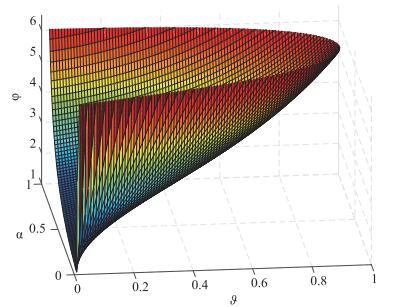
| \begin{align}\label{E38} \psi \left( {{\vartheta _i}, {\alpha _i}} \right) = \frac{{{{\left( {{\vartheta _i} + \left( {1 - {\vartheta _i}} \right){\alpha _i}} \right)}^2}}}{{\vartheta _i^2\left( {1 - {{\left( {{\vartheta _i} + \left( {1 - {\vartheta _i}} \right){\alpha _i}} \right)}^2}} \right){{\left( {1 - {\alpha _i}} \right)}^2}}}. \end{align} | (38) |
where the local parameters \left( {{\vartheta _i}, {\alpha _i}} \right) \in \left( {0, 1} \right) \times \left( {0, 1} \right). Figure 1 shows the graph of the function \psi \left( {{\vartheta _i}, {\alpha _i}} \right). From Fig. 1, we learn that the infimum of \psi ({{\vartheta _i}, {\alpha _i}}) is 1. Next, we prove it by the theoretical analysis.
Note that 1 - {\left( {{\vartheta _i} + \left( {1 - {\vartheta _i}} \right){\alpha _i}} \right)^2} < 1, then we have
| \begin{align}\label{E39} \psi \left( {{\vartheta _i}, {\alpha _i}} \right) > {\psi _1}\left( {{\vartheta _i}, {\alpha _i}} \right) = \frac{{{{\left( {{\vartheta _i} + \left( {1 - {\vartheta _i}} \right){\alpha _i}} \right)}^2}}}{{\vartheta _i^2{{\left( {1 - {\alpha _i}} \right)}^2}}}. \end{align} | (39) |
In the following, for the value \alpha_i, we divide three cases to consider.
For the first case {\alpha _i} \in \left( {0, 1} \right), we have
| \begin{align}\label{E40} &\; \psi \left( {{\vartheta _i}, {\alpha _i}} \right) > {\psi _1}\left( {{\vartheta _i}, {\alpha _i}} \right)\nonumber\\ &\; > \frac{{{{\left( {{\vartheta _i} + \left( {1 - {\vartheta _i}} \right){\alpha _i}} \right)}^2}}}{{\vartheta _i^2}} = {\left( {1 + \frac{{\left( {1 - {\vartheta _i}} \right){\alpha _i}}}{{{\vartheta _i}}}} \right)^2} > 1. \end{align} | (40) |
For the second case {\alpha _i} \to 1, it yields:
| \begin{align}\label{E41} &\; \mathop {\lim }\limits_{{\alpha _i} \to 1} \psi \left( {{\vartheta _i}, {\alpha _i}} \right) \nonumber\\ &\; = \mathop {\lim }\limits_{{\alpha _i} \to 1} \frac{{{{\left( {{\vartheta _i} + \left( {1 - {\vartheta _i}} \right){\alpha _i}} \right)}^2}}}{{\vartheta _i^2\left( {1 - {{\left( {{\vartheta _i} + \left( {1 - {\vartheta _i}} \right){\alpha _i}} \right)}^2}} \right){{\left( {1 - {\alpha _i}} \right)}^2}}} \to + \infty. \end{align} | (41) |
For the third case {\alpha _i} \to 0, we have
| \begin{align}\label{E42} &\;\mathop {\lim }\limits_{{\alpha _i} \to 0} \psi \left( {{\vartheta _i}, {\alpha _i}} \right)\nonumber\\ &\; = \mathop {\lim }\limits_{{\alpha _i} \to 0} \frac{{{{\left( {{\vartheta _i} + \left( {1 - {\vartheta _i}} \right){\alpha _i}} \right)}^2}}}{{\vartheta _i^2\left( {1 - {{\left( {{\vartheta _i} + \left( {1 - {\vartheta _i}} \right){\alpha _i}} \right)}^2}} \right){{\left( {1 - {\alpha _i}} \right)}^2}}}\nonumber\\ &\;= \frac{1}{{\left( {1 - \vartheta _i^2} \right)}} > 1. \end{align} | (42) |
Besides, note that \mathop {\lim }\limits_{{\vartheta _i} \to 0, {\kern 1pt} {\kern 1pt} {\alpha _i} \to 0} \psi \left( {{\vartheta _i}, {\alpha _i}} \right) = 1.
From (40)-(42), we obtain that the infimum of \psi ({{\vartheta _i}, {\alpha _i}}) is 1. Hence, by (37), the optimal variance as follows:
| \begin{align}\label{E43} {J^*} = \mathop {\inf }\limits_{{q_i}, {\beta _i}} J\left( {{q_i}, {\alpha _i}} \right) = 2{\delta ^2}d\mathop {\min }\limits_{{\vartheta _i}, {\alpha _i}} \sum\nolimits_{i = 1}^N {\frac{1}{{\varepsilon _i^2}}}, \end{align} | (43) |
which implies that the results of Theorem 4 hold.
In this subsection, we aim to confirm the theoretical results we have obtained based on the proposed algorithm (2). For the sake of convenience, we consider a undirected and connected ring network [47] with 20 agents. In all the simulations, we set \delta=0.7.
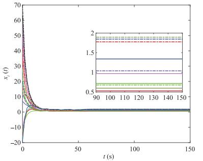
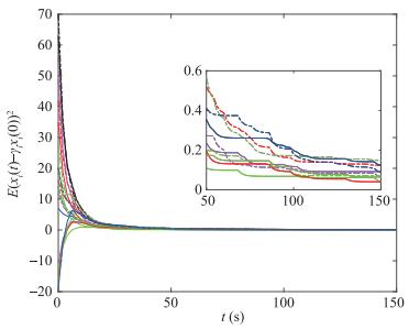
Fig. 3 shows that all network agents eventually reach certain values under algorithm (2) with parameters \alpha_i=0.8 and \beta_i=0.07. It can be found that all network agents do not converge to the same value, which implies that the network agents cannot converge to the exact average initial value. The result is in accordance with Proposition 4.1 in [31]. Fig. 4 depicts that all network agents eventually converge to the weighted average initial value in the mean square. The ETC algorithm parameters are set \alpha_i=0.8, \beta_i=0.07, \sigma_i=0.3 and the weighted value \gamma_i=10 for \forall i. The simulation testifies the results of Theorems 1 and 2.
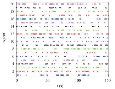
In order to illustrate the effectiveness of our event-triggered scheme, we present the ETC trajectory u_i(t) of all network agents in Fig. 5 with u_i(t)=\sum\nolimits_{j \in {N_i}} {{a_{ij}}{\theta _j}\left( {t_k^j} \right)}. The ETC algorithm parameters are set \alpha_i=0.8, \beta_i=0.07, \sigma_i=0.3 and the weighted value \gamma_i=10 for \forall i. It can be found that u_i(t) is the piecewise constant communication control function, which means that the communication among agents is discontinuous. Besides, Fig. 6 shows the event-triggered time instant of all network agents 1-20. Following Fig. 4, the event-triggered time instant further verify that the communication among agents is intermittent and just occurs at event-triggered time instant.
From the D section of Main results, it is found that there exists a trade-off between {\rm{var}}\left( {\sum\nolimits_{s = 0}^\infty {\tilde w\left( s \right)} } \right) and \epsilon_i with Laplace noise parameters c_i=0.7 and q_i=0.9. Fig. 7 shows the relationship between {\rm{var}}\left( {\sum\nolimits_{s = 0}^\infty {\tilde w\left( s \right)} } \right) and \epsilon_i, as is shown in (33). The result of Fig. 7 are in accordance with our conclusion.
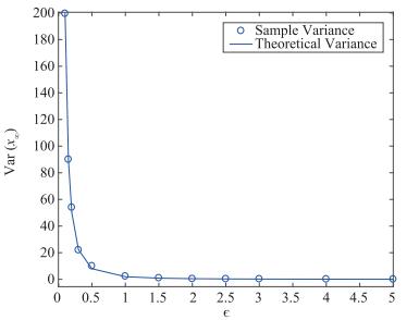
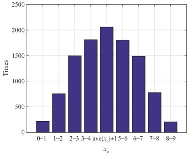
Fig. 8 depicts the histogram of convergence points for 10^4 times simulations under algorithm (2) with x_\infty=\bar x\left( 0 \right)+{\rm{var}}\left( {\sum\nolimits_{s = 0}^\infty {\tilde w\left( s \right)} } \right). The most of the convergence point are near the weighted average initial value. The distribution of the convergence point is similar to the Gaussian distribution. As we increase the simulation times, the distribution of the convergence point will approach closer to a Gaussian distribution function.
This paper aims to develop a new event-triggered update law for all agents in MANSs as our differentially private consensus algorithm. The results show that our proposed algorithm not only guarantees to achieve the consensus of all agents in MANSs, but also preserves the privacy of each agent' initial state against the other all agents. By the theoretical analysis, the sufficient condition of convergence and its accuracy are derived, respectively. Meanwhile, the differential privacy of the algorithm is guaranteed. Besides, the optimal solution to minimize the variance of the agents' convergence point according to the tradeoff between privacy and performance of our proposed algorithm is derived for the given privacy level. Finally, a numerical simulation example is used to testify the of the validity of our algorithm.
From the above conclusion, the convergence rate is not provided, which is due to the generality of the algorithm parameters. It is as described in Remark 4. This motivates us to improve our algorithm (2) such that we can derive the convergence rate. Besides, some interesting open questions left by this paper include expanding main results to switching topology directed graphs, the time-delay case and proposing the more effective privacy-preserving scheme for more general systems under the event-triggered communication strategy.
| [1] |
A. Shariati and Q. Zhao, "Robust leader-following output regulation of uncertain multi-agent systems with time-varying delay, " IEEE/CAA J. Autom. Sinica, vol. 5, no. 4, pp. 807-817, 2018. doi: 10.1109/JAS.2018.7511141
|
| [2] |
R. Olfati-Saber, J. A. Fax, and R. M. Murray, "Consensus and cooperation in networked multi-agent systems, " Proceedings of the IEEE vol. 95, no. 1, pp. 215-233, 2007. http://d.old.wanfangdata.com.cn/OAPaper/oai_arXiv.org_1009.6050
|
| [3] |
R. W. Beard, T. W. McLain, M. A. Goodrich, and E. P. Anderson, "Coordinated target assignment and intercept for unmanned air vehicles, " IEEE Transactions on Robotics and Automation, vol. 18, no. 6, pp. 911-922, 2002. doi: 10.1109/TRA.2002.805653
|
| [4] |
J. A. Fax and R. M. Murray, "Information flow and cooperative control of vehicle formations, " IEEE Transactions on Automatic Control, vol. 49, no. 9, pp. 1465-1476, 2004. doi: 10.1109/TAC.2004.834433
|
| [5] |
Q. Song, F. Liu, G. Wen, J. Cao, and X. Yang, "Distributed positionbased consensus of second-order multiagent systems with continuous/intermittent communication, " IEEE Transactions on Cybernetics, 2017. http://europepmc.org/abstract/MED/28436912
|
| [6] |
G. Wen, W. Yu, Z. Li, X. Yu, and J. Cao, "Neuro-adaptive consensus tracking of multiagent systems with a high-dimensional leader, " IEEE Transactions on Cybernetics, vol. 47, no. 7, pp. 1730-1742, 2017. doi: 10.1109/TCYB.2016.2556002
|
| [7] |
Z. Ji, H. Lin, and H. Yu, "Protocols design and uncontrollable topologies construction for multi-agent networks, " IEEE Transactions on Automatic Control, vol. 60, no. 3, pp. 781-786, 2015. doi: 10.1109/TAC.2014.2335971
|
| [8] |
A. Wang, T. Dong, and X. Liao, "On the general consensus protocol in multi-agent networks with second-order dynamics and sampled data, " Asian Journal of Control, vol. 18, no. 5, pp. 1914-1922, 2016. doi: 10.1002/asjc.1261
|
| [9] |
M. Yu, C. Yan, D. Xie, and G. Xie, "Event-triggered tracking consensus with packet losses and time-varying delays, " IEEE/CAA J. Autom. Sinica, vol. 3, no. 2, pp. 165-173, 2016. doi: 10.1109/JAS.2016.7451104
|
| [10] |
J. Wu, V. Ugrinovskii, and F. Allgöwer, "Cooperative estimation and robust synchronization of heterogeneous multi-agent systems with coupled measurements, " IEEE Transactions on Control of Network Systems 2017. http://ieeexplore.ieee.org/abstract/document/8003378/
|
| [11] |
M. S. Mahmoud and G. D. Khan, "LMI consensus condition for discretetime multi-agent systems, " IEEE/CAA J. Autom. Sinica, doi: 10.1109/JAS.2016.7510016, 2016.
|
| [12] |
W. He, B. Zhang, Q.-L. Han, F. Qian, J. Kurths, and J. Cao, "Leaderfollowing consensus of nonlinear multiagent systems with stochastic sampling, " IEEE Transactions on Cybernetics, vol. 47, no. 2, pp. 327-338, 2017. http://ieeexplore.ieee.org/document/7407343/
|
| [13] |
H. Zhang, T. Feng, G.-H. Yang, and H. Liang, "Distributed cooperative optimal control for multiagent systems on directed graphs: An inverse optimal approach, " IEEE Transactions on Cybernetics, vol. 45, no. 7, pp. 1315-1326, 2015. doi: 10.1109/TCYB.2014.2350511
|
| [14] |
S. Yang, Q. Liu, and J. Wang, "Distributed optimization based on a multiagent system in the presence of communication delays, " IEEE Transactions on Systems, Man, and Cybernetics: Systems, vol. 47, no. 5, pp. 717-728, 2017. doi: 10.1109/TSMC.2016.2531649
|
| [15] |
W. Ren, R. W. Beard, and E. M. Atkins, "A survey of consensus problems in multi-agent coordination, " in Proc. IEEE American Control Conference, 2005, pp. 1859-1864. https://www.researchgate.net/publication/224617178_A_Survey_of_Consensus_Problems_in_Multiagent_Coordination
|
| [16] |
C. Wang, X. Wang, and H. Ji, "A continuous leader-following consensus control strategy for a class of uncertain multi-agent systems, " IEEE/CAA J. Autom. Sinica, vol. 1, no. 2, pp. 187-192, 2014. doi: 10.1109/JAS.2014.7004549
|
| [17] |
H. Zhang, H. Jiang, Y. Luo, and G. Xiao, "Data-driven optimal consensus control for discrete-time multi-agent systems with unknown dynamics using reinforcement learning method, " IEEE Transactions on Industrial Electronics, vol. 64, no. 5, pp. 4091-4100, 2017. doi: 10.1109/TIE.2016.2542134
|
| [18] |
Q. Liu and J. Wang, "A second-order multi-agent network for boundconstrained distributed optimization, " IEEE Transactions on Automatic Control, vol. 60, no. 12, pp. 3310-3315, 2015. doi: 10.1109/TAC.2015.2416927
|
| [19] |
J. Qin, W. Fu, W. X. Zheng, and H. Gao, "On the bipartite consensus for generic linear multiagent systems with input saturation, " IEEE Transactions on Cybernetics, 2017. http://ieeexplore.ieee.org/document/7588177/
|
| [20] |
W. Hu, L. Liu, and G. Feng, "Output consensus of heterogeneous linear multi-agent systems by distributed event-triggered/self-triggered strategy, " IEEE Transactions on Cybernetics, 2017. http://www.ncbi.nlm.nih.gov/pubmed/27608484
|
| [21] |
X. Xu, L. Liu, and G. Feng, "Consensus of heterogeneous linear multiagent systems with communication time-delays, " IEEE Transactions on Cybernetics, 2017. http://europepmc.org/abstract/MED/28541918
|
| [22] |
Y. Khazaeni and C. G. Cassandras, "Event-driven trajectory optimization for data harvesting in multi-agent systems, " IEEE Transactions on Control of Network Systems, 2017. http://www.wanfangdata.com.cn/details/detail.do?_type=perio&id=Arxiv000001373882
|
| [23] |
J. Le Ny and G. J. Pappas, "Differentially private filtering, " IEEE Transactions on Automatic Control, vol. 59, no. 2, pp. 341-354, 2014. doi: 10.1109/TAC.2013.2283096
|
| [24] |
M. H. DeGroot, "Reaching a consensus, " Journal of the American Statistical Association, vol. 69, no. 345, pp. 118-121, 1974. doi: 10.1080/01621459.1974.10480137
|
| [25] |
N. E. Manitara and C. N. Hadjicostis, "Privacy-preserving asymptotic average consensus, " in Proc. IEEE European Control Conference, 2013, pp. 760-765. https://www.researchgate.net/publication/261498453_Privacy-preserving_asymptotic_average_consensus
|
| [26] |
Y. Mo and R. M. Murray, "Privacy preserving average consensus, " IEEE Transactions on Automatic Control, vol. 62, no. 2, pp. 753-765, 2017. doi: 10.1109/TAC.2016.2564339
|
| [27] |
X. Duan, J. He, P. Cheng, Y. Mo, and J. Chen, "Privacy preserving maximum consensus, " in Proc. IEEE 54th Confelence on Decision and Control, 2015, pp. 4517-4522. http://www.researchgate.net/publication/304411214_Privacy_Preserving_Maximum_Consensus
|
| [28] |
Z. Huang, S. Mitra, and G. Dullerud, "Differentially private iterative synchronous consensus, " in Proc. ACM Workshop on Privacy in the Electronic Society, 2012, pp. 81-90.
|
| [29] |
X. Wang, J. He, P. Cheng, and J. Chen, "Differentially private maximum consensus, " IFAC-PapersOnLine, vol. 50, no. 1, pp. 9509-9514, 2017. doi: 10.1016/j.ifacol.2017.08.1597
|
| [30] |
E. Nozari, P. Tallapragada, and J. Cort'es, "Differentially private average consensus with optimal noise selection, " IFAC-PapersOnLine, vol. 48, no. 22, pp. 203-208, 2015. doi: 10.1016/j.ifacol.2015.10.331
|
| [31] |
E. Nozari, P. Tallapragada, and J. Cort'es, "Differentially private average consensus: Obstructions, trade-offs, and optimal algorithm design, " Automatica, vol. 81, pp. 221-231, 2017. doi: 10.1016/j.automatica.2017.03.016
|
| [32] |
E. Garcia and P. J. Antsaklis, "Model-based event-triggered control for systems with quantization and time-varying network delays, " IEEE Transactions on Automatic Control, vol. 58, no. 2, pp. 422-434, 2013. doi: 10.1109/TAC.2012.2211411
|
| [33] |
X. Meng and T. Chen, "Event detection and control co-design of sampled-data systems, " International Journal of Control, vol. 87, no. 4, pp. 777-786, 2014. doi: 10.1080/00207179.2013.857047
|
| [34] |
A. Wang, T. Dong, and X. Liao, "Event-triggered synchronization strategy for complex dynamical networks with the markovian switching topologies, " Neural Networks, vol. 74, pp. 52-57, 2016. doi: 10.1016/j.neunet.2015.11.002
|
| [35] |
X. Meng and T. Chen, "Event based agreement protocols for multi-agent networks, " Automatica, vol. 49, no. 7, pp. 2125-2132, 2013. doi: 10.1016/j.automatica.2013.03.002
|
| [36] |
T. Dong and A. Wang, "Event-triggered consensus of nonlinear multiagent systems with unknown external disturbance, " Asian Journal of Control, 2018. doi: 10.1002/asjc.1682/full
|
| [37] |
A. Wang, X. Liao, and T. Dong, "Event-driven optimal control for uncertain nonlinear systems with external disturbance via adaptive dynamic programming, " Neurocomputing, 2017. http://cn.bing.com/academic/profile?id=a3593cc51b7c7621054923c7f56a8694&encoded=0&v=paper_preview&mkt=zh-cn
|
| [38] |
D. Wang, H. He, X. Zhong, and D. Liu, "Event-driven nonlinear discounted optimal regulation involving a power system application, " IEEE Transactions on Industrial Electronics, vol. 64, no. 10, pp. 8177-8186, 2017. doi: 10.1109/TIE.2017.2698377
|
| [39] |
D. Wang, H. He, and D. Liu, "Improving the critic learning for eventbased nonlinear h1control design, " IEEE Transactions on Cybernetics, vol. 47, no. 10, pp. 3417-3428, 2017. doi: 10.1109/TCYB.2017.2653800
|
| [40] |
D. Wang and D. Liu, "Learning and guaranteed cost control with eventbased adaptive critic implementation, " IEEE Transactions on Neural Networks and Learning Systems, 2018. http://ieeexplore.ieee.org/document/8336507/
|
| [41] |
Q. Zhang, D. Zhao, and D. Wang, "Event-based robust control for uncertain nonlinear systems using adaptive dynamic programming, " IEEE Transactions on Neural Networks & Learning Systems, vol. 29, no. 1, pp. 37-50, 2016. http://europepmc.org/abstract/MED/27775539
|
| [42] |
Y. Zhu, D. Zhao, H. He, and J. Ji, "Event-triggered optimal control for partially-unknown constrained-input systems via adaptive dynamic programming, " IEEE Transactions on Industrial Electronics, vol. 64, no. 5, pp. 4101-4109, 2017. doi: 10.1109/TIE.2016.2597763
|
| [43] |
Q. Zhang, D. Zhao, and Y. Zhu, "Event-triggered h control for continuous-time nonlinear system via concurrent learning, " IEEE Transactions on Systems, Man, & Cybernetics: Systems, vol. PP, no. 99, pp. 1-11, 2016. http://ieeexplore.ieee.org/document/7442588/
|
| [44] |
L. Gao, S. Deng, and W. Ren, "Differentially private consensus with event-triggered mechanism, " IEEE Transactions on Control of Network Systems, 2018. http://ieeexplore.ieee.org/document/8264765/
|
| [45] |
W. Xiong, X. Yu, R. Patel, and W. Yu, "Iterative learning control for discrete-time systems with event-triggered transmission strategy and quantization, " Automatica, vol. 72, pp. 84-91, 2016. doi: 10.1016/j.automatica.2016.05.031
|
| [46] |
R. Durrett, Probability: Theory and Examples. Cambridge University press, 2010.
|
| [47] |
J. F. Kurose, Computer Networking: A Top-down Approach Featuring the Internet. Addison-wesley, pp. 1-11, 2002.
|
| [1] | Chi Ma, Dianbiao Dong. Finite-time Prescribed Performance Time-Varying Formation Control for Second-Order Multi-Agent Systems With Non-Strict Feedback Based on a Neural Network Observer[J]. IEEE/CAA Journal of Automatica Sinica, 2024, 11(4): 1039-1050. doi: 10.1109/JAS.2023.123615 |
| [2] | Honghai Wang, Qing-Long Han. Designing Proportional-Integral Consensus Protocols for Second-Order Multi-Agent Systems Using Delayed and Memorized State Information[J]. IEEE/CAA Journal of Automatica Sinica, 2024, 11(4): 878-892. doi: 10.1109/JAS.2024.124308 |
| [3] | Meilin Li, Yue Long, Tieshan Li, Hongjing Liang, C. L. Philip Chen. Dynamic Event-Triggered Consensus Control for Input Constrained Multi-Agent Systems With a Designable Minimum Inter-Event Time[J]. IEEE/CAA Journal of Automatica Sinica, 2024, 11(3): 649-660. doi: 10.1109/JAS.2023.123582 |
| [4] | Zongyu Zuo, Jingchuan Tang, Ruiqi Ke, Qing-Long Han. Hyperbolic Tangent Function-Based Protocols for Global/Semi-Global Finite-Time Consensus of Multi-Agent Systems[J]. IEEE/CAA Journal of Automatica Sinica, 2024, 11(6): 1381-1397. doi: 10.1109/JAS.2024.124485 |
| [5] | Zhe Chen, Ning Li. An Optimal Control-Based Distributed Reinforcement Learning Framework for A Class of Non-Convex Objective Functionals of the Multi-Agent Network[J]. IEEE/CAA Journal of Automatica Sinica, 2023, 10(11): 2081-2093. doi: 10.1109/JAS.2022.105992 |
| [6] | Dan Zhang, Qiusheng Lian, Yueming Su, Tengfei Ren. Dual-Prior Integrated Image Reconstruction for Quanta Image Sensors Using Multi-Agent Consensus Equilibrium[J]. IEEE/CAA Journal of Automatica Sinica, 2023, 10(6): 1407-1420. doi: 10.1109/JAS.2023.123390 |
| [7] | Jingshu Sang, Dazhong Ma, Yu Zhou. Group-Consensus of Hierarchical Containment Control for Linear Multi-Agent Systems[J]. IEEE/CAA Journal of Automatica Sinica, 2023, 10(6): 1462-1474. doi: 10.1109/JAS.2023.123528 |
| [8] | Qing Yang, Gang Chen, Ting Wang. ADMM-based Distributed Algorithm for Economic Dispatch in Power Systems With Both Packet Drops and Communication Delays[J]. IEEE/CAA Journal of Automatica Sinica, 2020, 7(3): 842-852. doi: 10.1109/JAS.2020.1003156 |
| [9] | Zhenhua Wang, Juanjuan Xu, Huanshui Zhang. Consensus Seeking for Discrete-time Multi-agent Systems with Communication Delay[J]. IEEE/CAA Journal of Automatica Sinica, 2015, 2(2): 151-157. |
| [10] | Zhaoxia Wang, Minrui Fei, Dajun Du, Min Zheng. Decentralized Event-Triggered Average Consensus for Multi-Agent Systems in CPSs with Communication Constraints[J]. IEEE/CAA Journal of Automatica Sinica, 2015, 2(3): 248-257. |
| [11] | Wen Qin, Zhongxin Liu, Zengqiang Chen. Formation Control for Nonlinear Multi-agent Systems with Linear Extended State Observer[J]. IEEE/CAA Journal of Automatica Sinica, 2014, 1(2): 171-179. |
| [12] | Yi Dong, Jie Huang. Leader-following Rendezvous with Connectivity Preservation of Single-integrator Multi-agent Systems[J]. IEEE/CAA Journal of Automatica Sinica, 2014, 1(1): 19-23. |
| [13] | Hongbin Ma, Yini Lv, Chenguang Yang, Mengyin Fu. Decentralized Adaptive Filtering for Multi-agent Systems with Uncertain Couplings[J]. IEEE/CAA Journal of Automatica Sinica, 2014, 1(1): 101-112. |
| [14] | Airong Wei, Xiaoming Hu, Yuzhen Wang. Tracking Control of Leader-follower Multi-agent Systems Subject to Actuator Saturation[J]. IEEE/CAA Journal of Automatica Sinica, 2014, 1(1): 84-91. |
| [15] | Nan Xiao, Xuehe Wang, Lihua Xie, Tichakorn Wongpiromsarn, Emilio Frazzoli, Daniela Rus. Road Pricing Design Based on Game Theory and Multi-agent Consensus[J]. IEEE/CAA Journal of Automatica Sinica, 2014, 1(1): 31-39. |
| [16] | Chuanrui Wang, Xinghu Wang, Haibo Ji. A Continuous Leader-following Consensus Control Strategy for a Class of Uncertain Multi-agent Systems[J]. IEEE/CAA Journal of Automatica Sinica, 2014, 1(2): 187-192. |
| [17] | Chenghui Zhang, Le Chang, Xianfu Zhang. Leader-follower Consensus of Upper-triangular Nonlinear Multi-agent Systems[J]. IEEE/CAA Journal of Automatica Sinica, 2014, 1(2): 210-217. |
| [18] | Hongjing Liang, Huaguang Zhang, Zhanshan Wang, Junyi Wang. Consensus Robust Output Regulation of Discrete-time Linear Multi-agent Systems[J]. IEEE/CAA Journal of Automatica Sinica, 2014, 1(2): 204-209. |
| [19] | Hao Zhang, Gang Feng, Huaicheng Yan, Qijun Chen. Distributed Self-triggered Control for Consensus of Multi-agent Systems[J]. IEEE/CAA Journal of Automatica Sinica, 2014, 1(1): 40-45. |
| [20] | Wenhui Liu, Feiqi Deng, Jiarong Liang, Haijun Liu. Distributed Average Consensus in Multi-agent Networks with Limited Bandwidth and Time-delays[J]. IEEE/CAA Journal of Automatica Sinica, 2014, 1(2): 193-203. |

Figures(7)


Aijuan Wang, Xiaofeng Liao and Haibo He, "Event-Triggered Differentially Private Average Consensus for Multi-agent Network," IEEE/CAA J. Autom. Sinica, vol. 6, no. 1, pp. 75-83, Jan. 2019. doi: 10.1109/JAS.2019.1911327
 DownLoad:

 DownLoad:


