

Figure
1.
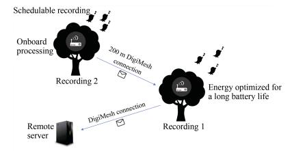
The proposed system architecture.
 Volume 6
Issue 1
Volume 6
Issue 1
IEEE/CAA Journal of Automatica Sinica
| Citation: | Zhengguo Sheng, Saskia Pfersich, Alice Eldridge, Jianshan Zhou, Daxin Tian and Victor C. M. Leung, "Wireless Acoustic Sensor Networks and Edge Computing for Rapid Acoustic Monitoring," IEEE/CAA J. Autom. Sinica, vol. 6, no. 1, pp. 64-74, Jan. 2019. doi: 10.1109/JAS.2019.1911324

|
Traditional biodiversity survey methods involve the identification and logging of species, by experts in-situ, based on what they see and hear at locations of interest. This implies several disadvantages like the vast amount of time and money to get constant results over a long period of time and a wide geographical distance, lack of reliability due to human error [1]. Based on the growing recognition of the ecological significance of the acoustic environment [2], passive acoustic monitoring is emerging as a promising solution to the urgent, global need for new biodiversity assessment methods. Two principle approaches to data collection currently exist: offline, programmable devices which require data to be periodically collected, and wireless sensor networks (WSN) which transmit raw audio files back to a central hub for acoustic analysis.
Offline devices require periodic collection of data which incurs extra labour and limits scalability in remote areas. Current WSN solutions do not include in situ monitoring and incur power consumption which obviates application in off-grid locations of key ecological interest. Although various WSN schemes have been developed to increase bandwidth efficiency [3], [4], sensor nodes are usually used for collecting data and there is a neglect of its computing capability and the potential benefits of being as a computing edge to process the data. The latest implementation of WSN based IoT [5], for accessing applications and services on wireless resource constrained networks 1 The typical wireless sensor device we consider is with limited processing speed to support IEEE 802.15.4-compliant radio transceiver., has enabled the newly emerging Sensor-as-a-cloud paradigm.
1 The typical wireless sensor device we consider is with limited processing speed to support IEEE 802.15.4-compliant radio transceiver.
In this paper, we propose a low cost solution for an audio recorder with onboard audio processing, embedded in a wireless sensor network based on a ZigBee protocol. The developed audio recorder can be used in several different use cases for which no cost effective, scalable biodiversity monitoring solution currently exists, such as to monitor pollinating insects, or to assess the condition of tropical forests by observing vocal animals [6], [7]. These use cases usually require a programming interface to schedule the recording times and change frequency according to application requirements and hardware constraints. As some areas are hard to access, the results are sent via a wireless interface to the server, so that no manual data collection is needed. Additionally, it is crucial to extend the battery life by an energy efficient use of the components. A fast Fourier transformation (FFT) to represent the audio signal in parallel to the recording saves memory and time and enables the system to efficiently generate and send acoustic indices to the server using a mesh network. A proof of concept of a cost efficient acoustic sensor network consisting of two nodes (recorders) and one server is also demonstrated and assessed for biodiversity monitoring. The main contribution of this paper is the following:
1) We develop an energy efficient wireless sensor network for remote audio recording and onboard processing. The low cost solution shows comparable performance to expensive commercial products in terms of audio quality. Moreover, wireless communications can further enable the capability of remote and real time monitoring.
2) We introduce the concept of edge computing and propose an effective computing strategy for an in/situ rapid acoustic survey. The test results show that up to 84% energy consumption can be saved using the local processing capability provided by senor node itself.
3) We show that the proposed wireless sensor networks can achieve acoustic equivalence and superior performance over current solutions at a much lower cost. The proposed edge computing strategy will be further deployed and tested in real application scenarios, such as forest reserve.
The remainder of the paper is the following: Section Ⅱ provides a brief overview of current technologies related to wireless sensor networks, acoustic signal processing and commercial solutions. Section Ⅲ describes the proposed system hardware architecture and software implementation. The justification of the system, especially the evaluation of acoustic equivalence, energy consumption and performance, are described in Section Ⅳ. Section Ⅴ summarizes the findings of this paper and gives recommendations for future developments.
Technologies for remote biodiversity monitoring have several advantages over traditional field survey methods: they are more efficient in cost and time, minimise habitat disturbance, remove human error and inter-observer variation, and provide permanent data records for future analyses [8]. There is a growing interest in rapid acoustic survey and numerous studies point to the potential for automated computational analysis of acoustic data, or acoustic indices, as a reliable and efficient method to support biodiversity monitoring (e.g. [7], [9]-[11]). Wireless acoustic sensor networks are already used in several applications, however there is no commercial device combining both approaches to compute acoustic indices in situ. Although doing so means the loss of permanent audio records, the gains are considerable: remote acoustic monitoring has potential to revolutionise biodiversity monitoring in signalling ecologically important changes, as well as providing a proxy for biodiversity, over spatio-temporal scales which are currently impossible to assess. However many of the regions of critical ecological importance are remote and without electrical grid, presenting a significant technical challenge to the development of large scale acoustic sensor networks [12]: the current approach of transmitting the raw audio recordings obviates long-term deployment in off-grid locations. Taking inspiration from current trends in network computing, we propose a power-efficient and cost-effective solution which computes indices in situ, vastly reducing the data transmission load and therefore bringing power consumption in line with battery or solar powered remote installation.
The Internet of Things (IoT) is an emerging technology which leads to significant changes in the way devices interact with each other [13]. Wireless sensor networks (WSNs) are one technology to enable the Internet of Things. Embedded electronics, sensors, software, and a network interface allows them to communicate with each other [14]. Sensors are usually used to measure temperature, pressure, and sound, whereas the microcontroller computes, analyses and coordinates the communication with other nodes [15].
WSNs have three main challenges: the power supply, node management and the network topology [16]. As the nodes are often distributed in a wide area with sometimes restricted access and powered through batteries, it is important to design them to be as power efficient as possible. Power efficiency does not only relate to the power supply, but it is a relevant characteristic in the whole development process, from the choice of hardware to the management and transmission of data [16]. Another significant criterion is the management of the remotely operating nodes, as they must operate unattended and with restricted access. The possibility to remotely configure the nodes and to implement them so they can organize themselves is crucial, e.g. to find another communication route when one route is not accessible [17], [18]. The third main challenge is the network topology, which can be implemented with a mesh network. Short distances between nodes are more power efficient during the transmission than long distances [19]. A mesh network topology, where nodes act as relays and as routers, gives the required flexibility and reliable communication [15].
These features of WSNs make it a suitable protocol for remote acoustic sensor networks. In studies where data over a wide range are required, WSNs are a cost and time efficient alternative, especially as device power efficiency increase and memory requirements drop [20]. Smart WSNs are not only able to collect large volumes of data associated with frequent sampling and/or long duration deployment, they are also able to process and filter the data according to application requirements, which otherwise would be a very time consuming and costly process [21]. This allows collection of data with programmable sampling regimes, over long time periods, without the need to deploy experts in the field [22] whilst also minimising habitat disturbance. The reducing costs and improving quality of sensors, batteries and microcontrollers accelerate the realization of WSNs for biodiversity. In this paper, we apply WSN in acoustic monitoring, particularly, with focus on the local computing capability of sensor node on calculating acoustic indices.
Traditional biodiversity surveys are carried out by experts in situ: species are identified and the tiem and location of their appearance logged [23]. The intense research of indices for the usage of biodiversity assessment has been doing in the last 30 years and is a complementary method for biodiversity studies [11]. The basic form of using the technology is to record data, i.e., audio files in this paper. Raw audio files generate vast volumes of data which need to be collected and manually processed with corresponding software tools [24]. The next step is to process and filter the data directly on nodes in the field, which gives the opportunity to send only the result [8]. In addition to the transmission time, this method will also accelerate the complete data collection and analysis process.
Different techniques focus on different kinds of audio analysis: one approach is to use machine learning to attempt to recognise specific species calls, however in tropical areas where species are not all known, this is complex, and even in temperate zones with fewer species, separation of individual calls from a wider acoustic scene is non-trivial and has not yet be reliably achieved in the wild [25]. An alternative is to survey the entire acoustic community within the broader acoustic environment or soundscape, and use acoustic indices which aim to provide proxies for more general biodiversity metrics such as species diversity of abundance [9], [26].
Background noises from wind, humans, or planes are a challenging interference factor for acoustic indices, because they can distort the results and must therefore be considered carefully [11]. Several filters and methods can be used to mitigate the effect of noise, e.g. amplitude threshold cut-off filters or downstream methods and spectrum subtraction [27], [28]. Dozens of indices have been proposed to date [29]. For illustration purposes, we implement the acoustic complexity index (ACI), as it is reported to be relatively insensitive to non-intermittent sounds such as airplane noise with constant intensity character [11], [30]. The ACI can be used to monitor bird songs under different environmental conditions as it positively correlates with the singing activity of birds [9]. The basis for the acoustic indices computation is a fast Fourier transformation (FFT). Each signal can be represented as a sum of several sine functions and its time domain will be transformed into the frequency domain which is required for the frequency analysis [31]. Using a window, depending on the application either Hanning or Hamming, reduces the disruptions at the changeover to the next frequency bin [31].
The ACI at each frequency area is calculated as an average of the absolute magnitude changes (D) and is divided by the sum of all values of intensity (Ik) over the number of time fractions (n) [9]
| ACI=Dk=1∑nIk. | (1) |
Commercial solutions for biodiversity assessment based on sound recording are available on the market. The Solo System [32], [33] is basically an instruction of suggested parts which have to be bought, assembled and prepared with a provided operating system. The functionality is restricted to the recording of sounds, which will be stored on the SD card. As the operating system is an open source file, it is completely customizable and can be extended with further functionalities like a wireless interface. However, onboard processing for audio files based on a FFT spectrogram would not be feasible due to hardware restrictions of the Raspberry Pi A (see Section Ⅲ-B1).
Soundscape Explorer Terrestrial [34] is the only device with an acoustic signal processing. The device can calculate the ACI in real-time, but as the other solutions, lacks a wireless communication interface. Further acoustic indices cannot be calculated with this solution. The battery pack lasts for about two weeks which allows a schedule of 1 minute recording and 5 minutes pause.
The high-end product in this comparison is the SM3 from Wildlife Acoustics [35]. Although it is a closed system it is highly customizable in terms of recording times, recording configuration and accessories used with the system. Wildlife Acoustics offers software to analyse the audio files, the SM3 itself does not process the data. Due to the missing wireless communication interface, the recorded data are stored on a SD card and no transmission to the server is intended. The SM3 will be used as a comparison to the developed recorder in [28].
Fig. 1 illustrates the proposed system architecture with its requirements. Each recorder consists of a Teensy microcontroller including a SD card, an audio board, a microphone, XBee module, and a battery in a waterproof case. The composition of these modules regarding their functional range, performance, energy consumption and costs is justified in Section Ⅲ-B. Instead of two fully equipped recorders, as illustrated in Fig. 1, we use one device to record and process the data, and another device, to relay messages only.
Each device can be individually configured to a user-defined recording schedule and executes onboard processing tasks, which prevents the need to save the audio files. Only the calculated acoustic indices are sent to the server in a multi-hop fashion, so that no data collection or external processing are required. Each XBee module automatically searches the fastest path to the server and relays the message. A detailed description of the software implementation is given in Section Ⅲ-C.
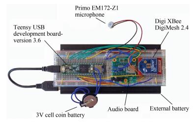
This section describes the motivation for each component in the wireless recorder, which is illustrated in Fig. 2. Using Digimesh, each node is a recorder and a router at the same time and therefore only one type of setup is needed for the nodes in the field. The total cost for one node is £ 97.10, without battery.
1) Computing Board and Wireless Communication Interface: Apart from the technical facts of different development boards, the support and availability of tested libraries are also a relevant consideration in hardware selection. We prefer to use development boards supporting a built-in digital signal processor (DSP) module due to its significant increases in performance [36]. The earliest version which supports a built-in DSP module is the ARM Cortex M4 [37]. Another important feature is the real-time clock (RTC), which is required to get the correct time of the recordings. In addition, the RTC can be used to wake up the board from sleep mode.
The powerful core in combination with a very efficient energy consumption, high flexibility in terms of enabling/disabling modules, and the low material cost, justify the decision to use a Teensy version 3.6 for the system development. A 3V cell coin battery is added to retain the date and time while the power is off (e.g. when the main battery is empty). To connect the nodes and cover a wide recording area, a mesh network with routers in between the nodes is a very efficient solution. Furthermore, the transmission power and the cost of the module is relevant for the decision. The XBee module has been chosen as the wireless interface, because it meets the requirements related to the range and the supported network topology, and is well supported with a dedicated library for the Teensy development board [38]-[40].
Digi have developed a proprietary mesh network protocol, Digimesh, which is based on ZigBee, but with the feature that no dedicated routing device is required. Each node can act as a node, a controller and a router which makes the network more flexible and no predefined route is required [41].
The Digimesh module is available in a standard variation and in a PRO variation. The PRO module has an extended range, but consumes more transmission power [41]. For the first tests and to verify which module fits best to the application the standard module is used. A compatible pinout and the usage of the same protocol allows it to exchange the module at a later stage if needed [40], [42].
2) Audio Interface: To add a high quality 16-bit audio to the Teensy, an audio board is used, which supports a 44.1 kHz sample rate [43]. It allows connecting stereo headphones to listen to the audio files and mono as well as stereo input for the recordings. The selected microphone is a single input microphone with a signal to noise ratio of 80 dB [44]. To reduce the background noise and to protect the Primo EM172-Z1 microphone, a windshield can be mounted over the microphone.
The audio library, which includes the FFT functionality, runs on the microcontroller of the Teensy and not on the microcontroller of the audio board. This means that the audio add-on board is only used for the connection and configuration of the microphone and to achieve the higher sample rate. The audio board supports a lot more functionalities, such as playing several audio files at the same time, mixing sound files, and adding special effects. A potential to further save cost and energy would be to develop a personalized add-on board, which only supports the required functionality instead of the full audio package.
3) Protection Case: As the design of the case is not focus of this paper, a plastic box with a hole for the microphone was used for field testing. The final case should be weather and shock-resistant, small and light to attach it easily in the trees and camouflage designed to protect it from theft. To prepare the case for future improvements the possibility to attach a solar panel should be given.
During the setup of a node, some low-level configurations are necessary to execute, specifically the setting of the time and the configuration of the XBee module. The XBee modules need to be configured to communicate in the same network, enable the sleep mode and adjust the power. Configurations and commands can easily be executed at the initial setup with direct access to the modules and using a graphical user interface or at a later stage using remote commands.
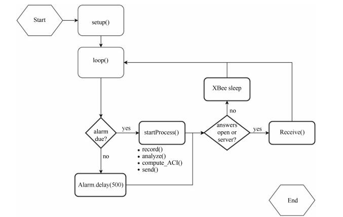
After the setup of the device, the loop function will be endless called. Each time an alarm is triggered and the startProcess() function is called. Within the function, four steps are executed: Firstly the recording of the data, then the analysis, followed by the ACI calculation. The last step is the send function of the calculated value.
For testing purposes, there is the option to store the recorded audio data on the SD card for further analysis. Otherwise only the calculated FFT spectrogram is stored on the SD card and a message with the ACI value is generated to send it to the server. After the successful transmission of the calculated acoustic index, the device will be set to sleep mode until the next alarm is due.
Within this implementation the spectrogram array is stored on the SD card and is read line by line for the ACI computation. Another possibility is to calculate the ACI value during the real-time generation of the spectrogram. In this later case it would not be necessary to save the spectrogram at all and this would improve the system performance. A reference for the ACI value implemented in Python and runs on a Raspberry Pi can be found from [45]. A program coded in the scripting language Python takes about five to ten times longer than a comparable program coded in the interpreted language C++ [46]-[49]. Furthermore, the required memory space for a Python program is almost double than that required for a C++ program [48]. Nevertheless, the developed Python code is a very good example to verify the results of the C++ coded FFT spectrogram and indices calculations.
For the wireless communication, each node is equipped with a XBee S2C module supporting Digimesh. The benefit of Digimesh is that each node can act as an end node, controller, and router. Using Acknowledge messages enables the system to verify the sending status. If the sending is successful, the node is set to sleep mode to save energy consumption and frees up the space in the message array. Otherwise the message will be resent up to five times and will worst case be stored on its own SD card. The message is limited to 73 Bytes and consists of the header with an identifier, a timestamp and the final acoustic indices [40].
In the wireless sensor network, the battery capacity of the deployed sensors is usually limited. Energy management is one of the most important design issues for the energy-hungry sensors, which significantly affects the overall performance of the network. Thus, an appropriate mechanism is needed to decide when to perform edge computing locally on an edge node or when to implement computation offloading from the edge node to the remote central server. To propose a decision-making policy for edge computing, we adopt two parameters to characterize the profile of a computing task or an application (i.e., acoustic signal processing) that needs to be processed: the size of the data file related to the computing task, L, and the application completion deadline, T. In addition, T is expressed as a positive integer denoting the maximum number of time slots that are required to process the computing task. According to much existing literature such as [50], [51], when performing the edge computing, i.e., the local processing, the optimal energy consumption of the CPU hardware that implements an optimal clock-frequency scheduling in each CPU cycle of the chip via the dynamic voltage scaling (DVS) technology [52] can be approximated by the following formula
| Ec=KL3T2 | (2) |
where the constant K is a scalable factor that reflects the computation energy per CPU cycle as well as the possibility that the CPU is able to complete the computing task by a given deadline. K can be tuned according to field measurements obtained in actual implementation.
Moreover, we consider to model the energy consumption of the wireless transmission between the source sensor to the remote server when assuming that the data file is offloaded to the server for the central computing. Here, for simplicity, we do not consider the additional energy cost incurred by the central processing in the server while focusing on evaluation of the energy consumption from the communication perspective. Let the hop number of propagating the data file to the central server be M and the channel state be g. According to exiting study [53], since the physical layer and media access control of the sensor node adopts the IEEE 802.15.4-based ZigBee protocol, the communication energy cost incurred in both transmit and receive modes of the sensor in a time slot can be approximated by an empirical monomial function as follows
| Ek=ρlnkg | (3) |
where ρ is the communication energy coefficient and lk denotes the size of the data bits transmitted in the k-th time slot. n is the order of monomial ranging within [1], [5]. Considering that the maximum number of the time slots to complete the computation offloading is T and the hop number is M, we can further derive the total communication energy consumption as
| Et=Mρ(LT)ngT=MρgLnTn−1. | (4) |
Let the speed of processing the computation task be λ=LT. Based on the above models (2) to (4), we can establish the following rules as the decision-making policy for edge computing and central computing, the goal of which is to achieve energy-efficient management:
1) If λ>(gKMρ)1n−3 and n≠3 or if MρgK>1 and n=3, Et>Ec always holds such that the sensors should perform edge computing;
2) If λ≤(gKMρ)1n−3 and n≠3 or if MρgK≤1 and n=3, Et≤Ec always holds such that the sensors should perform computation offloading for central computing.
The rules can be proven by comparing the computation energy cost Ec with the communication energy cost Et.
To explore the potential for the above described device in ecoacoustic monitoring, we evaluated the prototype node according to audio fidelity and equivalence of ecoacoustic metrics, energy efficiency, spatial range and temporal performance as follows.
To compare the developed recorder to a commercial product, two tests have been done with the SM3 from Wildlife Acoustics. The tests focus on the audio quality, rather than battery life or other factors. The test tones and environmental recordings are played back via a pair of gain-balanced Genelec 2030 s (standard studio acoustic monitors with a flat frequency response). Each device is positioned at a distance of 1.2 m from each speaker, in the same plane.
For the first test, sinusoidal test tones at different frequencies are played back in the sound proofed studio to demonstrate the clarity of hardware in the system.
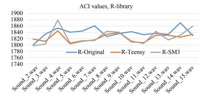
In the second test, a series of 14 environmental recordings with differing levels of acoustic activity (UK dawn chorus) are played back in a soundproofed studio. Each sound file is 1 minute long and has previously been labelled by species richness values (number of distinct species heard per minute) and all relevant indices have been calculated, using the Python Acoustic Indices library, which in turn has been validated against Seewave and soundecology packages in R-library (version 3.3.3) [45]. The sound files are recorded with the Teensy and the SM3, and their indices are also calculated and compared. As a reference value, the ACI is calculated based on the original file, the.wav file from the SM3 and the converted.raw from the Teensy file using the R-library.
The result of this test shows that, the ACI values calculated using the Teensy implementation with a FFT1024 are approximately doubled compared to the calculated values by the R-library (FFT512). Using the same FFT1024 window, the values calculated by the Python implementation are very close to the values calculated by the Teensy. There is only a minimal variation with a maximum of 10%, but the general trend, which is illustrated in Fig. 4, is the same.
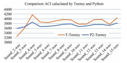
Differences between results from the Teensy and the Python implementation can be due to different input methods. The Python and R-library read out the audio files whereas the Teensy plays back the audio files and makes a real-time FFT1024 calculation. This means that the spectrogram generation of the Teensy is dependent on the internal audio instruments, which calculate the spectrogram based on a recording and not the already generated audio file content. Another difference can be due to round-off errors, which can occur during the spectrogram generation and the ACI calculation.
The first ACI value (Sound 2.wav), displayed in Fig. 4, is conspicuous as the discrepancy is particularly large. As both calculations are based on the same recording, the reason cannot be due to the microphone or other recording instruments. The recording itself is very quiet and the one with the fewest bird activities. This leads to small magnitude changes in the spectrogram and can therefore be more affected by the round-off errors than spectrograms with higher magnitude changes.
Comparing the absolute differences of the ACI values based on the different recorders and the same library (R-library), we show that the audio quality of the Teensy recordings is slightly better than the SM3 recordings. Fig. 5 shows the behaviour of the recordings compared to the original audio files which have been played back.
So far we have proved that it is possible to use a low budget development board for audio recording and in situ analysis. In this section we demonstrate that this method is more efficient than sending the audio file to the remote server and doing centralized signal processing with more powerful software and hardware tools.
The energy consumption for the transmission of a 1 min audio raw file can be estimated based on the values from the Teensy & XBee data sheets [40]:
| Transmission time=size audio filedata rate=42600bits250kbs=170.4s | (5) |
| Energy consumption=Energy XBee+Energy Teensy=2.13mAh+4.06mAh=6.19mAh. | (6) |
To transmit a 1 min audio raw file, 6.26 mAh are needed using the highest power level to achieve the maximum range [40]. This value includes only the energy consumption for the transmission of the file, the external audio processing on the server is not considered in this calculation. As a comparison, an onboard ACI calculation of a 1 min audio raw file in addition to the transmission of the calculated acoustic index takes 0.84 mAh (based on measurements, see Section Ⅳ-C2). Although this comparison is only an estimation, it clearly demonstrates the energy savings of 86% using onboard processing.
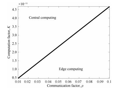
To illustrate how the computation and the communication factors affect the energy efficiency when the energy-efficient decision-making policy is employed, we set the size of the data file as L=73×8bits and the completion deadline as T=100ms (the duration of each time slot is 2ms). The channel gain is specified as g=0.5. According to the real measurements reported in [54], the computation factor K ranges in the order of 10−11 and the communication factor ρ is in the order of 10−2. M is set to M=2 as the two-hop routing is adopted for data transmission, and n is set to n=4. Fig. 6 shows the energy-efficient region with respect to the computation and the communication factors, K and ρ, under the edge computing and the central computing. From this figure, it is easy to determine the best strategy to process the computing task.
To enable operations in remote areas, wireless nodes need to be powered by battery and/or solar power. As the implementation has an impact on the energy consumption of the system, different power saving strategies need to be considered. Furthermore, the energy consumption of the system needs to be determined under different recording schedules.
1) Power Saving Mode: There are different options to reduce the energy consumption of the system [55]:
a) Sleep mode of XBee: The XBee is set to sleep mode when not in use (e.g. during the recording). It will be woken up at the beginning of the send and receive function and set to sleep mode afterwards on pin transition. This saves 31-45 mAh, compared to the receive or transmit execution of the XBee [40].
b) Sleep mode of Teensy: Using the Snooze.h library [56] enables the Teensy to enter low power mode. The relevant function of the library is to wake up the Teensy after a specific period by using the RTC to keep the time and wake up the Teensy on pin transition. Using only the Teensy and the XBee, the Snooze.h library works as expected and the current drops to below 1mA.
c) Disabling unused peripherals: Disabling unused modules such as USB and Analog to Digital Converter also saves power, the latter saving approximately 0.8 mA [57]. In this study, the Teensy is powered over the USB interface, as this is a convenient method to use a power bank. But for the future work, it needs to be determined if it is more efficient to use the USB interface only for the node configuration and power the node in the field with a battery pack directly connected to the pins 3.3 V and GND.
2) Energy Consumption: As a first step, the power consumption of the individual features is measured. The results are based on an 1h operation mode and are measured with an USB digital power meter.
a) Recorder in sleep mode: <1 mAh
b) Recorder in IDLE mode: 86.3 mAh
c) 1 min recording: 1.43 mAh
d) ACI calculation (approx. 30 s): 0.84 mAh
e) Send/receive call:
Best case (successful transmission-1.4 s): 0.18 mAh
Worst case (6 resend attempts-71.2 s): 2.17 mAh
Using a schedule of a 1 min recording every 10 minutes between 4 am-9 am and 5 pm to 10 pm results in a total energy consumption of 147.3 mAh in case the sleep mode is set during off time and a 2087 mAh in case the device goes only into IDLE mode. Table Ⅰ shows the total energy consumption of the test using the proposed edge computing and central computing (transmission only), respectively.
| Schedule (1 min every 10 min) | Total 24 h (4 am to 9 am, 5 pm to10 pm) | Edge computing | Central comp. (trans. only) |
| Recording | 10 h × 6 recordings/h | 86 mAh | 86 mAh |
| ACI calculation | 10 h × 6 calculations/h | 50.4 mAh | 0 |
| Transmission (Best case) | 10 h × 6 transmit/h | 10.8 mAh | 375.6 mAh |
| Idle mode | 1349 min | 1940 mAh | 1940 mAh |
| Total energy consumption | 2087.2 mAh | 2401.6 mAh | |
 DownLoad:
CSV
DownLoad:
CSV
The central computing includes only the energy consumption for the transmission of the file (to the server), the external audio processing on the remote server is not considered in the calculation. It is clear that the edge computing approach can reduce the overall energy consumption. If we compare the ACI processing and transmission alone, the energy consumption can be saved by 83.7%. This schedule is only one example of dynamic power management and the calculations have been verified running it for 24 h without a full sleep mode, as there is still a problem with the usage of the Snooze.h library.
This arbitrary model shows that the Teensy has significant power savings in comparison to current solutions, e.g. during recording 20% compared to the Solo System and up to 280% compared to the SM3 [32], [35].
So far what we have done is to implement a simple (up to 2 hops) ZigBee mesh network as a proof the concept. ZigBee is a physical layer technique that has proven energy efficiency in single hop transmission. However, in practise, we need to cope with a large-scale network coverage by developing a multi-hop mesh IoT network. Moreover, multi-tasking is also needed not only for monitoring and collecting acoustic data, but also remotely maintaining and configuring IoT devices. Therefore, development of higher layer networking and application protocols is necessary to achieve system level energy efficiency for large scale mesh network. The latest IETF protocol stack (6LowPAN/IPv6/UDP/CoAP) has defined the routing and application protocols for Low power and Lossy Networks to facilitate the multi-hop connectivity. In our latest work [58], we have successfully shown energy efficiency and reliability of the proposed protocol stack using simulation tool. In our future work, we will further develop such multi-hop mesh network prototype and verify its energy performance in practise.
For the XBee S2C module a range of up to 1200 m is defined in the specification with the usage of different antenna [40]. The module in this study uses an implemented wire antenna connected directly to the PCB with a gain of 1.5-1.8 dbi [59]. There are further options with other integrated antenna or connectors for external antenna to improve the antenna gain and the maximum distance between two nodes.
Using the integrated antenna, two different power configurations are set to measure the maximum distance where a reliable communication between three nodes should be maintained.
The first configuration uses the lowest power level and a disabled boost mode resulting in a stable communication up to 25 m between the two end nodes, i.e., recorder 1 and 2 in Fig. 1. The second test is configured with the highest power level and an enabled boost mode and had a stable communication up to 110 m between the two end nodes. Both tests have been executed with a line of sight between the nodes and under the same weather conditions (18∘C, 40 km/h wind, 70% air humidity and 120 m above zero).
To extend the range to the required 200 m either the XBee PRO module needs to be used or an antenna. Both options need further investigation, which are recommended for future developments on the system.
To determine the system performance, several functions are measured. The execution time to measure the time impacts the system and is therefore only implemented for the tests. Test setup:
a) 100 repetitions for each sending case
b) 1 minute of recording
c) Spectrogram calculation and storage on the SD card
d) Calculation of ACI
e) Sending message to the server, with six resend attempts if needed and storage on the SD card
f) Point-to-point communication and WSN with three nodes
In this performance measurement, the message array overflow will not be considered in the overall system performance as the scenario is very unlikely and highly dependent on the scheduled interval. A message overflow can happen when the alarm interval is higher than the total resending time. In such a case, the message needs to be stored on the SD card.
The average values of the 100 repetitions are summarized as follows:
The performance tests show that the FFT spectrogram calculation only needs 1.8 s longer than the recording itself and the ACI calculation is approximately 50% of the recording time. A 1-minute recording including the acoustic index calculation and the transmission of the result within a three-node network to the server only takes 91.5 s in the best case where the message is received by the server within the first sending attempt. Decreasing the total execution time of 91.5 s by the length of the recording time itself leads to an extra effort of 31.5 s. This highlights the huge time benefit of using a WSN for biodiversity compared to recording devices, where data need to be manually collected and analysed.
| Calculation of FFT spectrogram | 61.8 s |
| Calculation of ACI value | 28.3 s |
| Sending of messages (Point-to-Point) | Best Case: 1.1 s |
| Worst Case: 71.2 s | |
| Sending of messages (3 nodes with 2 hops) | Best Case: 1.4 s |
| Worst Case: 71.2 s |
DownLoad:
CSV
To improve the performance of the ACI calculation, the implementation can be changed to calculate the ACI in real time with the recording and spectrogram generation rather than from the finalized and stored spectrogram. This would save the time it needs to read the spectrogram line by line. It needs to be determined how this would affect acoustic indices, which are based on different spectrogram parameters. The Soundscape Explorer Terrestrial promotes this real-time calculation of the ACI without considering other acoustic indices [34].
The conclusion and the recommendations for further research are presented as follows.
Passive acoustic monitoring is emerging as potential solution for cost-effective biodiversity monitoring, however offline battery powered devices limit scalability and the transmission of raw audio data is too power intensive for many remote, off-grid sites of ecological interest. In this paper, we have proposed the combination of in situ analyses and transmission of ecoacoustic indices rather than raw audio using a wireless sensor network. A prototype device built from lost cost hardware was described and evaluated for audio performance, energy efficiency, spatial range and temporal performance. These benchmark tests showed acoustic equivalence, both in raw signal and calculation of example ecoacoustic metric, and considerable power savings of up to 280% during the recording time compared to current leading commercial offline solutions. Range test and power tests demonstrate the prototype is suitable for extended deployment in densely forested areas, of typical conservation concern. Temporal tests show that an acoustic index of a 1 min recording can arrive at the server only 30 s after the recording has finished, affording near real-time performance which could be of great value in tracking endangered species, or identifying illegal activity such as logging or poaching in protected areas.
The following recommendations are under the assumption that the onboard processing based approach is more efficient than the remote processing based approach, i.e., by sending the computed acoustic indices to the server rather than the complete audio file.
1) For the proof of concept only one acoustic index has been calculated, but for a comprehensive acoustic analysis, further indices are required. The implementation and testing, especially regarding the limited memory, should be investigated for future work.
2) To improve the system's efficiency the ACI value can be calculated during the FFT generation, and without saving the spectrogram on the SD card. This would save some operating time and the node can go to sleep mode earlier.
3) An entire sleep mode of the system needs to be implemented as this has a huge impact on the battery life. Additionally, the integration of solar as a second power source should be considered for a long-lasting operation.
4) To improve the audio quality and to reduce the costs, the breadboard needs be replaced by soldering the components and keeping the crucial audio wires as short as possible. As the recorders are meant to be deployed in a larger area, there is the need to build a large number of nodes and test the mesh network functionality.
5) As already suggested in Section Ⅳ-D, the range between the nodes can be extended using another antenna. A detailed analysis to identify the balance between range and power consumption might be an interesting topic for future enhancements of the wireless recorders.
| [1] |
A. Gasc, J. Sueur, S. Pavoine, R. Pellens, and P. Grandcolas, "Biodiversity sampling using a global acoustic approach: contrasting sites with microendemics in new caledonia, " PLoS One, vol. 8, no. 5, e65311, 2013. doi: 10.1371/journal.pone.0065311
|
| [2] |
J. Sueur and A. Farina, "Ecoacoustics: The ecological investigation and interpretation of environmental sound, " Biosemiotics, vol. 8, no. 3, pp. 493-502, 2015. doi: 10.1007/s12304-015-9248-x
|
| [3] |
N. Correia, D. Sacramento, and G. Schutz, "Dynamic aggregation and scheduling in coap/observe-based wireless sensor networks, " IEEE Internet of Things Journal, vol. 3, no. 6, pp. 923-936, Dec. 2016.
|
| [4] |
M. F. Brejza, L. Li, R. G. Maunder, B. M. Al-Hashimi, C. Berrou, and L. Hanzo, "20 years of turbo coding and energy-aware design guidelines for energy-constrained wireless applications, " IEEE Communications Surveys Tutorials, vol. 18, no. 1, pp. 8-28, 2016. doi: 10.1109/COMST.2015.2448692
|
| [5] |
Z. Sheng, H. Wang, C. Yin, X. Hu, S. Yang, and V. C. M. Leung, "Lightweight management of resource-constrained sensor devices in internet of things, " IEEE Internet of Things Journal, vol. 2, no. 5, pp. 402-411, Oct. 2015.
|
| [6] |
D. Goulson, A Sting in the Tale. Random House, 2016.
|
| [7] |
A. Eldridge, M. Casey, P. Moscoso, and M. Peck, "A new method for ecoacoustics? Toward the extraction and evaluation of ecologicallymeaningful soundscape components using sparse coding methods, " Peer J, vol. 4, e2108, 2016. doi: 10.7717/peerj.2108
|
| [8] |
R. S. Rempel, K. A. Hobson, G. Holborn, S. L. Van Wilgenburg, and J. Elliott, "Bioacoustic monitoring of forest songbirds: interpreter variability and effects of configuration and digital processing methods in the laboratory, " Journal of Field Ornithology, vol. 76, no. 1, pp. 1-11, 2005. doi: 10.1648/0273-8570-76.1.1
|
| [9] |
N. Pieretti, A. Farina, and D. Morri, "A new methodology to infer the singing activity of an avian community: the acoustic complexity index (aci), " Ecological Indicators, vol. 11, no. 3, pp. 868-873, 2011. doi: 10.1016/j.ecolind.2010.11.005
|
| [10] |
A. Gasc, J. Sueur, F. Jiguet, V. Devictor, P. Grandcolas, C. Burrow, M. Depraetere, and S. Pavoine, "Assessing biodiversity with sound: Do acoustic diversity indices reflect phylogenetic and functional diversities of bird communities?" Ecological Indicators, vol. 25, pp. 279-287, 2013. doi: 10.1016/j.ecolind.2012.10.009
|
| [11] |
M. Depraetere, S. Pavoine, F. Jiguet, A. Gasc, S. Duvail, and J. Sueur, "Monitoring animal diversity using acoustic indices: implementation in a temperate woodland, " Ecological Indicators, vol. 13, no. 1, pp. 46-54, 2012. doi: 10.1016/j.ecolind.2011.05.006
|
| [12] |
B. M. Napoletano, "Integrating biophony into biodiversity measurement and assessment, " Ecoacoustics: The Ecological Role of Sounds, pp. 169, 2017. doi: 10.1002/9781119230724.ch10/summary
|
| [13] |
Z. Sheng, S. Yang, Y. Yu, A. V. Vasilakos, J. A. Mccann, and K. K. Leung, "A survey on the ietf protocol suite for the internet of things: standards, challenges, and opportunities, " IEEE Wireless Communications, vol. 20, no. 6, pp. 91-98, Dec. 2013.
|
| [14] |
I. Lee and K. Lee, "The internet of things (iot): applications, investments, and challenges for enterprises, " Business Horizons, vol. 58, no. 4, pp. 431-440, 2015. doi: 10.1016/j.bushor.2015.03.008
|
| [15] |
F. Zhao, L. J. Guibas, and L. Guibas, Wireless Sensor Networks: an Information Processing Approach. Morgan Kaufmann, 2004.
|
| [16] |
W. Dargie and C. Poellabauer, Fundamentals of Wireless Sensor Networks: Theory and Practice. John Wiley & Sons, 2010.
|
| [17] |
A. Cerpa and D. Estrin, "Ascent: Adaptive self-configuring sensor networks topologies, " in Proc. INFOCOM 21st Annu. Joint Conf. IEEE Computer and Communications Societies. vol. 3. 2002, pp. 1278-1287.
|
| [18] |
K. L. Mills, "A brief survey of self-organization in wireless sensor networks, " Wireless Communications and Mobile Computing, vol. 7, no. 7, pp. 823-834, 2007. doi: 10.1002/(ISSN)1530-8677
|
| [19] |
G. J. Pottie and W. J. Kaiser, "Wireless integrated network sensors, " Communications of the ACM, vol. 43, no. 5, pp. 51-58, 2000. doi: 10.1145/332833.332838
|
| [20] |
J. Porter, P. Arzberger, H.-W. Braun, P. Bryant, S. Gage, T. Hansen, P. Hanson, C.-C. Lin, F.-P. Lin, T. Kratz, et al., "Wireless sensor networks for ecology, " AIBS Bulletin, vol. 55, no. 7, pp. 561-572, 2005. http://d.old.wanfangdata.com.cn/OAPaper/oai_doaj-articles_b54d3d1089230bf62a94d1e5d128f92e
|
| [21] |
S. L. Collins, L. M. Bettencourt, A. Hagberg, R. F. Brown, D. I. Moore, G. Bonito, K. A. Delin, S. P. Jackson, D. W. Johnson, S. C. Burleigh et al., "New opportunities in ecological sensing using wireless sensor networks, " Frontiers in Ecology and the Environment, vol. 4, no. 8, pp. 402-407, 2006. doi: 10.1890/1540-9295(2006)4[402:NOIESU]2.0.CO;2
|
| [22] |
C. wa Maina, "Audio diarization for biodiversity monitoring, " in Proc. 12th IEEE Africon International Conference-Green Innovation for African Renaissance, 2015, pp. 1-5.
|
| [23] |
W. H. Petraborg, E. G. Wellein, and V. E. Gunvalson, "Roadside drumming counts a spring census method for ruffed grouse, " The Journal of Wildlife Management, vol. 17, no. 3, pp. 292-295, 1953. doi: 10.2307/3797109
|
| [24] |
D. C. Marvin, L. P. Koh, A. J. Lynam, S. Wich, A. B. Davies, R. Krishnamurthy, E. Stokes, R. Starkey, and G. P. Asner, "Integrating technologies for scalable ecology and conservation, " Global Ecology and Conservation, vol. 7, pp. 262-275, 2016. doi: 10.1016/j.gecco.2016.07.002
|
| [25] |
A. Thessen, "Adoption of machine learning techniques in ecology and earth science, " One Ecosystem, vol. 1, e8621, 2016. doi: 10.3897/oneeco.1.e8621
|
| [26] |
R. Bardeli, D. Wolff, F. Kurth, M. Koch, K.-H. Tauchert, and K.-H. Frommolt, "Detecting bird sounds in a complex acoustic environment and application to bioacoustic monitoring, " Pattern Recognition Letters, vol. 31, no. 12, pp. 1524-1534, 2010. doi: 10.1016/j.patrec.2009.09.014
|
| [27] |
A. Farina and N. Pieretti, "Sonic environment and vegetation structure: a methodological approach for a soundscape analysis of a mediterranean maqui, " Ecological Informatics, vol. 21, pp. 120-132, 2014. doi: 10.1016/j.ecoinf.2013.10.008
|
| [28] |
A. Gasc, S. Pavoine, L. Lellouch, P. Grandcolas, and J. Sueur, "Acoustic indices for biodiversity assessments: analyses of bias based on simulated bird assemblages and recommendations for field surveys, " Biological Conservation, vol. 191, pp. 306-312, 2015. doi: 10.1016/j.biocon.2015.06.018
|
| [29] |
A. Eldridge, P. Guyot, P. Moscoso, A. Johnston, Y. Eyre-Walker, and M. Peck, "Sounding out ecoacoustic metrics: avian species richness is predicted by acoustic indices in temperate but not tropical habitats, " Ecological Indicators, vol. 95, pp. 939-952, 2018. doi: 10.1016/j.ecolind.2018.06.012
|
| [30] |
A. Farina, N. Pieretti, and L. Piccioli, "The soundscape methodology for long-term bird monitoring: A mediterranean europe case-study, " Ecological Informatics, vol. 6, no. 6, pp. 354-363, 2011. doi: 10.1016/j.ecoinf.2011.07.004
|
| [31] |
N. Instruments, "National instrument fundamentals, "[Online]. Available: http://download.ni.com/evaluation/pxi/Understanding%20FFTs%20and%20Windowing.pdf, Accessed on: Dec. 30, 2016.
|
| [32] |
R. C. Whytock and J. Christie, "Solo: an open source, customizable and inexpensive audio recorder for bioacoustic research, " Methods in Ecology and Evolution, vol. 8, no. 3, pp. 308-312, 2017. doi: 10.1111/2041-210X.12678
|
| [33] |
Solo, "Solo, "[Online]. Available: http://solo-system.github.io/home.html, Accessed on: Dec. 23, 2017.
|
| [34] |
S. Explorer, "Soundscape explorer, "[Online]. Available: http://iinsteco.org/soundscape_explorer/, Accessed on: Jan. 14, 2017.
|
| [35] |
I. Wildlife Acoustics, "Wildlife acoustics, "[Online]. Available: https://www.wildlifeacoustics.com/products/song-meter-sm3, Accessed on: Jan. 14, 2017.
|
| [36] |
A. E. Media, "Arm developer, "[Online]. Available: https://developer.arm.com/academia/armedumedia/online-courses/digital-signal-processing, Accessed on: Jan. 1, 2017.
|
| [37] |
ARM, "Arm, "[Online]. Available: http://infocenter.arm.com/help/topic/com.arm.doc.ddi0439b/DDI0439B_cortexm4_r0p0_trm.pdf, Accessed on: Dec. 22, 2009.
|
| [38] |
Adafruit, "Introducing the adafruit bluefruit le uart friend, "[Online]. Available: https://learn.adafruit.com/introducing-the-adafruit-bluefruit-le-uart-friend/downloads, Accessed on: Sep. 29, 2016.
|
| [39] |
PJRC, "Pjrc, "[Online]. Available: https://www.pjrc.com/teensy/td_libs_XBee.html, Accessed on: Jan. 1, 2017.
|
| [40] |
Digi, "Xbee/xbee-pro digimesh 2.4, "[Online]. Available: https://www.digi.com/resources/documentation/digidocs/pdfs/90001506.pdf, Accessed on: Jan. 1, 2017.
|
| [41] |
R. Faludi, Building Wireless Sensor Networks: with ZigBee, XBee, Arduino, and Processing. O'Reilly Media, Inc., 2010.
|
| [42] |
Digi, "Digi xbee digimesh 2.4, "[Online]. Available: https://www.digi.com/products/xbee-rf-solutions/2-4-ghz-modules/xbee-digimesh-2-4#specifications, Accessed on: Jan. 1, 2017.
|
| [43] |
PJRC, "Pjrc, "[Online]. Available: https://www.pjrc.com/store/teensy3_audio.html, Accessed on: July 21, 2017.
|
| [44] |
F. C. Ltd, "Fel communications ltd microphone amplifiers, "[Online]. Available: http://www.micbooster.com/documents/EM172Z1%20July%202015.pdf, Accessed on: July 1, 2015.
|
| [45] |
P. Guyot, "Acoustic indices, "[Online]. Available: https://github.com/sandoval31/Acoustic_Indices, Accessed on: Mar. 5, 2017.
|
| [46] |
G. v. Rossum, "Comparing python to other languages, "[Online]. Available: https://www.python.org/doc/essays/comparisons/, Accessed on: Jan. 1, 2017.
|
| [47] |
L. Prechelt, "An empirical comparison of seven programming languages, " Computer, no. 10, pp. 23-29, 2000. http://www.wanfangdata.com.cn/details/detail.do?_type=perio&id=4c0c3e51bd319e66619885d003c876a0
|
| [48] |
M. Fourment and M. R. Gillings, "A comparison of common programming languages used in bioinformatics, " BMC Bioinformatics, vol. 9, no. 1, pp. 82, 2008. http://d.old.wanfangdata.com.cn/OAPaper/oai_doaj-articles_3b1146388986d1e2b7eb9d911783e1bc
|
| [49] |
A. Huang, "Comparison of programming performance: Promoting stem and computer science education, " in Integrated STEM Education Conference (ISEC), 2015, pp. 123-125.
|
| [50] |
W. Zhang, Y. Wen, K. Guan, D. Kilper, H. Luo, and D. O. Wu, "Energyoptimal mobile cloud computing under stochastic wireless channel, " IEEE Transactions on Wireless Communications, vol. 12, no. 9, pp. 4569-4581, Sept. 2013.
|
| [51] |
Z. Sheng, C. Mahapatra, V. C. M. Leung, M. Chen, and P. K. Sahu, "Energy efficient cooperative computing in mobile wireless sensor networks, " IEEE Transactions on Cloud Computing, vol. 6, no. 1, pp. 114-126, Jan. 2018.
|
| [52] |
J. M. Rabaey, A. P. Chandrakasan, and B. Nikolic, Digital Integrated Circuits. Prentice Hall Englewood Cliffs, 2002, vol. 2.
|
| [53] |
J. Lee and N. Jindal, "Delay constrained scheduling over fading channels: Optimal policies for monomial energy-cost functions, " in Proc. IEEE Int. Conf. Communications, June 2009, pp. 1- 5.
|
| [54] |
A. P. Miettinen and J. K. Nurminen, "Energy efficiency of mobile clients in cloud computing, " in Proc. 2nd USENIX Conference on Hot Topics in Cloud Computing, ser. HotCloud'10. Berkeley, CA, USA: USENIX Association, 2010, pp. 4.[Online]. Available: http://dl.acm.org/citation.cfm?id=1863103.1863107
|
| [55] |
M. Kooijman, Building Wireless Sensor Networks Using Arduino. Packt Publishing Ltd, 2015.
|
| [56] |
Github, "Teensy low power library: Snooze v6.3.2, "[Online]. Available: https://github.com/duff2013/Snooze, Accessed on: July 21, 2018.
|
| [57] |
PJRC, "Pjrc, "[Online]. Available: https://www.pjrc.com/store/teensy3_audio.html, Accessed on: July 21, 2017.
|
| [58] |
X. Liu, Z. Sheng, C. Yin, F. Ali, and D. Roggen, "Performance analysis of routing protocol for low power and lossy networks (RPL) in large scale networks, " IEEE Internet of Things Journal, vol. 4, no. 6, pp. 2172-2185, 2017. doi: 10.1109/JIOT.2017.2755980
|
| [59] |
Digi, "Knowledge base, "[Online]. Available: http://knowledge.digi.com/articles/Knowledge_Base_Article/Antenna-Connection/?l=en_US&c=Product_Category%3AXBee_DigiMesh_2_4&fs=RelatedArticle, Accessed on: Jan. 1, 2015.
|
| [1] | Haotian Xu, Shuai Liu, Yueyang Li, Ke Li. Distributed Observer for Full-Measured Nonlinear Systems Based on Knowledge of FMCF[J]. IEEE/CAA Journal of Automatica Sinica, 2025, 12(1): 69-85. doi: 10.1109/JAS.2024.124467 |
| [2] | Kang Xiong, Qinglai Wei, Hongyang Li. Residential Energy Scheduling With Solar Energy Based on Dyna Adaptive Dynamic Programming[J]. IEEE/CAA Journal of Automatica Sinica, 2025, 12(2): 403-413. doi: 10.1109/JAS.2024.124809 |
| [3] | Nianyin Zeng, Xinyu Li, Peishu Wu, Han Li, Xin Luo. A Novel Tensor Decomposition-Based Efficient Detector for Low-Altitude Aerial Objects With Knowledge Distillation Scheme[J]. IEEE/CAA Journal of Automatica Sinica, 2024, 11(2): 487-501. doi: 10.1109/JAS.2023.124029 |
| [4] | Zimo Yin, Jian Pu, Yijie Zhou, Xiangyang Xue. Two-Stage Approach for Targeted Knowledge Transfer in Self-Knowledge Distillation[J]. IEEE/CAA Journal of Automatica Sinica, 2024, 11(11): 2270-2283. doi: 10.1109/JAS.2024.124629 |
| [5] | Aditya Joshi, Skieler Capezza, Ahmad Alhaji, Mo-Yuen Chow. Survey on AI and Machine Learning Techniques for Microgrid Energy Management Systems[J]. IEEE/CAA Journal of Automatica Sinica, 2023, 10(7): 1513-1529. doi: 10.1109/JAS.2023.123657 |
| [6] | Zefeng Zheng, Luyao Teng, Wei Zhang, Naiqi Wu, Shaohua Teng. Knowledge Transfer Learning via Dual Density Sampling for Resource-Limited Domain Adaptation[J]. IEEE/CAA Journal of Automatica Sinica, 2023, 10(12): 2269-2291. doi: 10.1109/JAS.2023.123342 |
| [7] | Meiqin Tang, Jiawen Sheng, Shaoyan Sun. A Coverage Optimization Algorithm for Underwater Acoustic Sensor Networks based on Dijkstra Method[J]. IEEE/CAA Journal of Automatica Sinica, 2023, 10(8): 1769-1771. doi: 10.1109/JAS.2023.123279 |
| [8] | Zhi-Xin Liu, Xiao-Cao Jin, Yuan-Ai Xie, Yi Yang. Joint Slot Scheduling and Power Allocation in Clustered Underwater Acoustic Sensor Networks[J]. IEEE/CAA Journal of Automatica Sinica, 2023, 10(6): 1501-1503. doi: 10.1109/JAS.2022.106031 |
| [9] | Xinhua Wang, Shasha Zhao, Lei Guo, Lei Zhu, Chaoran Cui, Liancheng Xu. GraphCA: Learning From Graph Counterfactual Augmentation for Knowledge Tracing[J]. IEEE/CAA Journal of Automatica Sinica, 2023, 10(11): 2108-2123. doi: 10.1109/JAS.2023.123678 |
| [10] | Yutong Wang, Xiao Wang, Xingxia Wang, Jing Yang, Oliver Kwan, Lingxi Li, Fei-Yue Wang. The ChatGPT After: Building Knowledge Factories for Knowledge Workers with Knowledge Automation[J]. IEEE/CAA Journal of Automatica Sinica, 2023, 10(11): 2041-2044. doi: 10.1109/JAS.2023.123966 |
| [11] | Jun Mei, Zhenyu Lu, Junhao Hu, Yuling Fan. Energy-Efficient Optimal Guaranteed Cost Intermittent-Switch Control of a Direct Expansion Air Conditioning System[J]. IEEE/CAA Journal of Automatica Sinica, 2021, 8(11): 1852-1866. doi: 10.1109/JAS.2020.1003447 |
| [12] | Teng Liu, Bin Tian, Yunfeng Ai, Fei-Yue Wang. Parallel Reinforcement Learning-Based Energy Efficiency Improvement for a Cyber-Physical System[J]. IEEE/CAA Journal of Automatica Sinica, 2020, 7(2): 617-626. doi: 10.1109/JAS.2020.1003072 |
| [13] | Qiang Fan, Nirwan Ansari. On Cost Aware Cloudlet Placement for Mobile Edge Computing[J]. IEEE/CAA Journal of Automatica Sinica, 2019, 6(4): 926-937. doi: 10.1109/JAS.2019.1911564 |
| [14] | Zhen Hong, Rui Wang, Xile Li. A Clustering-tree Topology Control Based on the Energy Forecast for Heterogeneous Wireless Sensor Networks[J]. IEEE/CAA Journal of Automatica Sinica, 2016, 3(1): 68-77. |
| [15] | Hepeng Li, Chuanzhi Zang, Peng Zeng, Haibin Yu, Zhongwen Li. A Stochastic Programming Strategy in Microgrid Cyber Physical Energy System for Energy Optimal Operation[J]. IEEE/CAA Journal of Automatica Sinica, 2015, 2(3): 296-303. |
| [16] | Xiaoyuan Luo, Liu Feng, Jing Yan, Xinping Guan. Dynamic Coverage with Wireless Sensor and Actor Networks in Underwater Environment[J]. IEEE/CAA Journal of Automatica Sinica, 2015, 2(3): 274-281. |
| [17] | Zhixin Liu, Yazhou Yuan, Xinping Guan, Xinbin Li. An Approach of Distributed Joint Optimization for Cluster-based Wireless Sensor Networks[J]. IEEE/CAA Journal of Automatica Sinica, 2015, 2(3): 267-273. |
| [18] | Changqing Xia, Wei Liu, Qingxu Deng. Cost Minimization of Wireless Sensor Networks with Unlimited-lifetime Energy for Monitoring Oil Pipelines[J]. IEEE/CAA Journal of Automatica Sinica, 2015, 2(3): 290-295. |
| [19] | Xiaohua Xia, Jiangfeng Zhang. Operation Efficiency Optimisation Modelling and Application of Model Predictive Control[J]. IEEE/CAA Journal of Automatica Sinica, 2015, 2(2): 166-172. |
| [20] | Haiyang Yu, Yisha Liu, Wei Wang. Distributed Sparse Signal Estimation in Sensor Networks Using H∞-Consensus Filtering[J]. IEEE/CAA Journal of Automatica Sinica, 2014, 1(2): 149-154. |

Figures(6) / Tables(2)


Zhengguo Sheng, Saskia Pfersich, Alice Eldridge, Jianshan Zhou, Daxin Tian and Victor C. M. Leung, "Wireless Acoustic Sensor Networks and Edge Computing for Rapid Acoustic Monitoring," IEEE/CAA J. Autom. Sinica, vol. 6, no. 1, pp. 64-74, Jan. 2019. doi: 10.1109/JAS.2019.1911324
| Schedule (1 min every 10 min) | Total 24 h (4 am to 9 am, 5 pm to10 pm) | Edge computing | Central comp. (trans. only) |
| Recording | 10 h × 6 recordings/h | 86 mAh | 86 mAh |
| ACI calculation | 10 h × 6 calculations/h | 50.4 mAh | 0 |
| Transmission (Best case) | 10 h × 6 transmit/h | 10.8 mAh | 375.6 mAh |
| Idle mode | 1349 min | 1940 mAh | 1940 mAh |
| Total energy consumption | 2087.2 mAh | 2401.6 mAh | |
DownLoad:
CSV
| Calculation of FFT spectrogram | 61.8 s |
| Calculation of ACI value | 28.3 s |
| Sending of messages (Point-to-Point) | Best Case: 1.1 s |
| Worst Case: 71.2 s | |
| Sending of messages (3 nodes with 2 hops) | Best Case: 1.4 s |
| Worst Case: 71.2 s |
DownLoad:
CSV
| Schedule (1 min every 10 min) | Total 24 h (4 am to 9 am, 5 pm to10 pm) | Edge computing | Central comp. (trans. only) |
| Recording | 10 h × 6 recordings/h | 86 mAh | 86 mAh |
| ACI calculation | 10 h × 6 calculations/h | 50.4 mAh | 0 |
| Transmission (Best case) | 10 h × 6 transmit/h | 10.8 mAh | 375.6 mAh |
| Idle mode | 1349 min | 1940 mAh | 1940 mAh |
| Total energy consumption | 2087.2 mAh | 2401.6 mAh | |
| Calculation of FFT spectrogram | 61.8 s |
| Calculation of ACI value | 28.3 s |
| Sending of messages (Point-to-Point) | Best Case: 1.1 s |
| Worst Case: 71.2 s | |
| Sending of messages (3 nodes with 2 hops) | Best Case: 1.4 s |
| Worst Case: 71.2 s |
 DownLoad:

 DownLoad:


