

Figure
1.
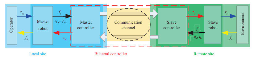
Structure and internal signal flow of teleoperation systems under the proposed composite controller
 Volume 6
Issue 5
Volume 6
Issue 5
IEEE/CAA Journal of Automatica Sinica
| Citation: | Zhenhua Zhao, Jun Yang, Shihua Li and Wen-Hua Chen, "Composite Nonlinear Bilateral Control for Teleoperation Systems With External Disturbances," IEEE/CAA J. Autom. Sinica, vol. 6, no. 5, pp. 1220-1229, Sept. 2019. doi: 10.1109/JAS.2018.7511273

|
Teleoperation denotes a local operator manipulates remote objects as if the operator were at the remote location [1]. The teleoperation systems extend a person's haptic and manipulation capability to a remote location [2], [3] and they are widely employed in the cases where humans are unable to perform a certain task [4] (e.g., outer space and undersea exploration, nuclear waste site and radioactive material management), or where human operators want to improve the semi-autonomous execution of a task [5] (e.g., minimally invasive telesurgery and telerehabilitation). As shown in Fig. 1, a teleoperation system usually consists of a human operator, a master robot, a slave robot, environment and communication channel. To perform a task in the remote environment, the human operator manipulates the master robot at local site, with appropriate control action in the master and slave robots (i.e., bilateral control action), the slave robot reproduces the master robot's motion at the remote site and the master robot displays the slave-environment contact force to the human operator. If the motions of the master and slave robots are the same and the contact force displayed by the master robot is the same as the slave-environment contact force, the ideal transparency is achieved [6].
To achieve high transparency in a teleoperation system, many bilateral control methods have been proposed. Based on the impedance control conception [7], the four-channel bilateral control architecture has been proposed in [6]. It achieves ideal transparency when master and slave robots are linear systems and no disturbances are imposed on them. To attenuate the influence of disturbance, the adaptive laws are designed to approximate the impedance model of teleoperation systems in [8], and the adaptive bilateral controller is developed based on the obtained impedance model. However, the disturbance attenuation ability is achieved at the price of sacrificing its nominal control performance [9].
To overcome the constraints of the above bilateral methods, the linear disturbance observer (LDOB) based bilateral control methods are developed in [10] and [11]. The LDOB based control method is an efficient way to deal with disturbance in linear motion control systems [12]. The oblique coordinate control (OCC) method in [10] employs LDOB in work space to estimate the lumped disturbances in master and slave robots, and then the disturbance estimations are utilized to compensate the disturbances in the master and slave robots such that they behave as the desired linear impedance model, and finally the OCC controller is developed based on the impedance model. To handle the couplings between the position and force tracking error dynamics in the OCC method, the diagonalization control (DC) method is proposed in [11] based on the concept of modal space disturbance observer (MDOB), where LDOB is designed in model space and utilized to estimate the disturbances and guarantee that the dynamics of system in modal space behave as linear dynamics. Then, the DC controller is constructed based on the estimation of MDOB and the nominal linear model. Although the above methods improve the transparency of teleoperation systems in different aspects, they all view the desired nominal model as linear impedance model. However, it is well known that, depending on the mechanical configuration, a robot may have strong nonlinear dynamics [13]. Although some weak nonlinearity may be considered as a part of disturbances and the above existing methods could be applied to yield satisfactory performance, dynamic performance and transparency in teleoperation systems degrade significantly when the master or slave robot exhibits strong nonlinearity.
To reduce the effects of nonlinear dynamics, a number of nonlinear bilateral control methods have been proposed recently [14], [15]. In general, these approaches can be classified into two categories including modal space based nonlinear method [14] and nonlinear dynamics based method [15]. In [14], system transparency is achieved through transferring the position and force control task into designing a nonlinear controller to guarantee the convergence of modal space states. However, the force control task usually cannot be satisfactorily achieved when master and slave robots have different dynamics. Nonlinear dynamics based method in [15] introduces a new way to design the bilateral controller, which designs the position tracking controller through nonlinear feedback directly based on the nonlinear dynamics of position tracking errors. However, to the best of our knowledge, only the tracking of position and velocity are considered in most of the existing nonlinear dynamics based methods.
Composite nonlinear control methods based on disturbance observers are efficient ways to handle disturbance and uncertainties in nonlinear systems [16] and they are widely studied in industrial process [17], [18] and flight control systems [19]. In this paper, a new composite nonlinear bilateral control method based on nonlinear disturbance observer (NDOB) [20] is proposed through the following steps. Firstly the position and force tracking error dynamics are obtained based on the nonlinear dynamics of the teleopeartion systems. Secondly, the NDOB is introduced to estimate the disturbances in the tracking error dynamics. Then, both the virtual position and force controllers are constructed based on the estimations of NDOB and nonlinear feedback methods. Finally, the virtual controllers are transformed into the real control actions of the master and slave robots through a nonlinear transformation. Careful comparisons with the existing methods have been conducted, it is shown that the proposed method has the following major merits: 1) convergence of both position and force tracking errors is ensured; 2) faster convergence rate and smaller steady-state error of position and force tracking errors are achieved.
The rest of the paper is organized as follows. The model and control objectives of teleoperation systems are given in Section Ⅱ. Section Ⅲ analyses three existing bilateral control methods and highlights the motivation of our work. In Section Ⅳ, a composite nonlinear bilateral controller based on NDOB is described in details. Performance of the proposed method is compared with some existing bilateral control methods in Section Ⅴ. Finally, conclusions are given in Section Ⅵ.
To demonstrate the conception of the bilateral control more clearly, the 1-degree-of-freedom bilateral systems are employed in this paper to derive the bilateral control methods. The nonlinear dynamics of master and slave robots with external disturbances in the joint space are given by [15]
| mm(qm)¨qm+cm(qm,˙qm)˙qm+gm(qm)+dm+τh=τmms(qs)¨qs+cs(qs,˙qs)˙qs+gs(qs)+ds+τe=τs | (1) |
where subscripts m and s denote master and slave robots respectively, qm, qs are the joint angle positions, mm(qm), ms(qs) are the inertias, cm(qm,˙qm), cs(qs,˙qs) include the Coriolis and centrifugal terms, gm(qm), gs(qs) are the gravity terms, dm, ds are the external disturbance torques which include the friction terms, τm, τs are the control torques, τh, τe are the external torques that the human operator applies to the master robot and the environment applies to the slave robot respectively. Considering that the robots are usually driven by electrical motors, the external torques and the end effector positions of 1-degree-of-freedom master and slave robots in the task space (Cartesian space) can be obtained through the following kinematics [21]
| τh=fhlm,τe=fels | (2) |
| xm=lmqm,˙xm=lm˙qm, xs=lsqs, ˙xs=ls˙qs | (3) |
where fh, fe denote the external interaction forces that the operator applies to the master and the environment applies to the slave, lm and ls are the distances between the shaft and the points where the contact forces are applied, xm and xs are the positions of master and slave. The interaction forces fh and fe are naturally specified in task space and they are usually modeled as mass spring dampers [10] and given by
| fh=frh−bh˙xm−kh(xm−xm0)fe=fre−be˙xs−ke(xs−xs0) | (4) |
where bh, kh, be and ke are positive constants, xm0 and xs0 are the balance positions where contact forces can be kept zero, and frh, fre are the exogenous forces of the human operator and the environment, respectively.
Remark 1: To demonstrate the conception of the prosed bilateral control method more clearly, only the 1-degree-of-freedom model is considered and employed to derive the composite controller. It should be noted that all the presented methods are effective to multi-degree-of-freedom bilateral systems and can be generalized to n-degree-of-freedom bilateral systems.
The control objective of the teleoperation systems is to realize the bilateral haptic transmission between the remote site and the local site. Human beings perceive the property of an environment object by touching the object and feeling its deformation and reaction force. Consequently, the haptic transmission objective of the bilateral systems can be specified as follows:
1) To transmit the human action and guarantee that the operator senses the deformation of remote environment, the positions of the master and slave robots should be the same
| eP=xm−xs→0. | (5) |
2) To perceive the reaction force of the environment, the force from the environment should be transmitted to the operator vividly when the slave robot contacts with environment
| eF=fh+fe→0. | (6) |
To promote the wide applications of bilateral systems, such as extending operator's ability by scaling local contact force to manipulate heavy loads or by zooming out local motions to perform delicate tasks, the above control objectives are usually transformed as follows:
| eP=xm−αxs→0, eF=fh+βfe→0 | (7) |
where α and β are scaling positive constants. It is obvious that when α=β=1, the control objectives (7) reduce to the control objectives (5) and (6).
The position dynamics of the master and slave robots in task space can be obtained from (1)-(3) as
| ¯mm(qm)¨xm=fm−fdM, ¯ms(qs)¨xs=fs−fdS | (8) |
with
| fdM= fh+cm(qm,˙qm)˙qm+gm(qm)+dmlmfdS= fe+cs(qs,˙qs)˙qs+gs(qs)+dslsfm= τmlm, fs=τsls, ¯mm=mm(qm)l2m, ¯ms=ms(qs)l2s |
where fm and fs are the force controllers of robots.
In the subsequent part, three well-known existing bilateral control methods which are designed based on the above dynamics are introduced and analysed. The motivation of our method is given to overcome these identified shortcomings.
Let positive constants ¯mmn and ¯msn represent the nominal constant parts of ¯mm(qm) and ¯ms(qs) in (8) respectively. The nominal linear model of (8) is given by
| ¯mmn¨xm=fm−fdm, ¯msn¨xs=fs−fds | (9) |
with
| fdm= fdM+(¯mm(qm)−¯mmn)¨xmfds= fdS+(¯ms(qs)−¯msn)¨xs. |
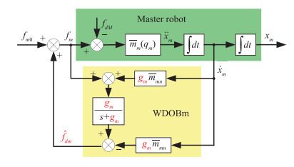
The disturbance observer in workspace (WDOB) [10] is introduced to estimate the lumped disturbance in (9). Take the WDOB design in the master robot workspace as an example, the design block diagram is given in Fig. 2. The disturbance estimation of WDOB can be calculated based on Fig. 2 as
| ˆfdm= gms+gm[fm+gm¯mmn˙xm]−gm¯mmn˙xmˆfds= gss+gs[fs+gs¯msn˙xs]−gs¯msn˙xs | (10) |
where gm, gs are the observer gains and they are designed as positive constants. To achieve the control objective of teleoperation systems in (7), the modal space states are introduced in [10] through the following transformation:
| ˜x=[˜xX˜xF]=[1−α1β][xmxs]=Jt[xmxs]˜fF=fh+βfe | (11) |
where ˜x is the state vector in modal space and Jt is a constant scaling matrix. The dynamics (9) can be transformed into the modal space based on (11) as
| ˜m¨˜x=Jt[fm−fdmfs−fds] | (12) |
with
| ˜m=Jt[¯mmn00¯msn]J−1t=[˜m11˜m12˜m21˜m22]. |
The final oblique coordinate control (OCC) law [10] is designed based on the above transformation as
| [fmfs]=J−1t[M1cP(s)˜xX+M2cF(s)˜fFcF(s)˜fF]+[ˆfdmˆfds] | (13) |
with
| M1=˜m11−˜m12˜m21˜m22, M2=˜m12˜m22 |
where ˆfdm and ˆfds are obtained from the WDOB (10), cP(s) and cF(s) are the feedback controller of position and force and they are usually designed as [10]
| CP(s)=−kPP−kPDs, CF(s)=kFbh | (14) |
where kPP, kPD and kF are positive constants.
Substituting the OCC law (13) into dynamics (12) yields the close-loop dynamics of bilateral systems:
| ¨˜xX=−kPP˜xX−kPD˙˜xX+˜e1M1−M2M1˜e2¨˜xF=kF˜m22bh˜fF−˜m21˜m22¨˜xX+1˜m22˜e2 | (15) |
with
| ˜e1=(ˆfdm−fdm)−α(ˆfds−fds) ˜e2=(ˆfdm−fdm)+β(ˆfds−fds). |
Combining (4) and (11) yields
| −bh¨˜xF= ˙˜fF−(˙frh+β˙fre)+(kh˙xm+βke˙xs)+β(be−bh)¨xs. | (16) |
Substituting (16) into (15) obtains the close-loop force tracking error dynamics under the OCC law (13) as
| ˙˜fF=−kF˜m22˜fF+bh(˜m21˜m22¨˜xX−1˜m22˜e2)+(˙frh+β˙fre)−β(be−bh)¨xs−(kh˙xm+βke˙xs). | (17) |
Remark 2: (15) and (17) imply that the force tracking error dynamics under the OCC law couple with the position tracking error dynamics. The couplings may degrade the static and dynamic features or even result in unstable control performance of the force tracking error subsystem.
An efficient solution to the coupling problem of the position and force tracking error dynamics in modal space is known as diagonalization control (DC) method [11]. With the transformation (11) in mind, the dynamics (8) can be transformed into the modal space as
| ¯m(qm,qs)¨˜x=Jt[fm−fdMfs−fdS] | (18) |
with
| ¯m(qm,qs)= Jt[¯mm(qm)00¯ms(qs)]J−1t= [¯m11¯m12¯m21¯m22]. |
Let us introduce the nominal dynamics of (18) as follows:
| [¯mXn00¯mFn]¨˜x=Jt[fmfs]−[fdXfdF] | (19) |
with
| [fdXfdF]=[(¯m11−¯mXn)¨˜xX+¯m12¨˜xF(¯m22−¯mFn)¨˜xF+¯m21¨˜xX]+Jt[fdMfdS] |
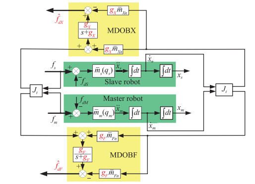
where ¯mXn and ¯mFn are the nominal values of ¯m11 and ¯m22 in (18) and they are chosen as positive constants. The MDOB [11] is designed based on the nominal linear dynamics (19) in model space as MDOBX and MDOBF which are shown in Fig. 3. The disturbance estimations of MDOB can be calculated based on Fig. 3 as
| [ˆfdXˆfdF]=G1(s)(Jt[fmfs]+G2(s)¯mn˙˜x)−G2(s)¯mn˙˜x | (20) |
with
| G1(s)= diag{gXs+gX, gFs+gF}G2(s)= diag{gX, gF} |
where ¯mn=diag{¯mXn,¯mFn}, and gX, gF are the observer gains of MDOBX and MDOBF, and they are designed as positive constants. The final diagonalization controller [11] is designed based on (19) as
| [fmfs]=J−1t[¯mXnCP(s)˜xX+ˆfdXCF(s)˜fF+ˆfdF] | (21) |
where ˆfdX and ˆfdF are obtained from MDOB (20), CP(s) and CF(s) are designed as (14).
Substituting the DC law (21) into the modal space dynamics (19) yields
| ¨˜xX=−kPP˜xX−kPD˙˜xX+ˆfdX−fdX¯mXn¨˜xF=kF¯mFnbh˜fF+ˆfdF−fdF¯mFn. | (22) |
Combining (16) and (22) obtains the close-loop force tracking error dynamics under the DC law (21) as
| ˙˜fF=−kF¯mFn˜fF−bh¯mFn(ˆfdF−fdF)+(˙frh+β˙fre)−β(be−bh)¨xs−(kh˙xm+βke˙xs). | (23) |
Remark 3: It follows from (22) that the DC method achieves the decoupling of force and position tracking error dynamics in modal space as desired. However, (23) implies that the force tracking error cannot be driven to the desired equilibrium point unless the steady-state states of systems are constants and disturbance fdF is accurately estimated.
Based on system dynamics (18) in modal space, the modal space based sliding mode control (MSSMC) method is proposed in [14]. The sliding variable is defined as
| σX=¨˜xX−CP(s)˜xX, σF=¨˜xF−CF(s)˜fF. | (24) |
The MSSMC law is designed as
| [fmfs]=J−1t¯m(qm,qs)[CP(s)˜xX−ηX∫σXdtCF(s)˜fF−ηF∫σFdt]. | (25) |
With (24) in mind, combining (18) and (25) yields
| [σX+ηX∫σXdtσF+ηF∫σFdt]+Jt[¯mm(qm)00¯ms(qs)]−1[fdMfdS]=0. |
Once the sliding variables σX and σF converge to zero, combining (14), (16) and (24), we have the close-loop dynamics of position and force tracking errors as follows:
| ¨˜xX=−kPP˜xX−kPD˙˜xX˙˜fF=−kF˜fF+(˙frh+β˙fre)−β(be−bh)¨xs−(kh˙xm+βke˙xs). | (26) |
Remark 4: Tracking performance of systems under the MSSMC method is not influenced by system's nonlinearities due to the utilization of nonlinear terms in controller (25). However the close-loop force tracking error dynamics (26) denotes this method cannot guarantee the force tracking error converge to zero unless the steady-state states of systems are constants. These will be shown in the later simulation comparison studies.
As shown by (17), (23) and (26), the force tracking error dynamics under the OCC law, the DC law and the MSSMC method are influenced by system states. All the above controllers alleviate the influences passively, where a controller cannot react directly and fast enough, although it can finally suppress the influences through feedback regulation in a relatively slow way [22].
To solve the coupling problem between force tracking error dynamics and system states such that the force tracking error has a satisfactory dynamic performance, we aim to address the problem through the following two steps: 1) Designing a baseline nonlinear feedback bilateral controller based on position and force tracking error nonlinear dynamics such that the position and force tracking error dynamics are decoupled from system states; 2) Constructing a composite nonlinear bilateral controller via introducing the estimation of disturbances based on NDOBs into the baseline controller to achieve fast disturbance rejection via a feedforward compensation way.
Let us define the position tracking error eP and force tracking error eF based on (7) as follows:
| eP=xm−αxs, eF=fh+βfe. | (27) |
The position tracking error dynamics can be obtained from (1)-(3) as
| ˙eP=lm˙qm−αls˙qs, ¨eP=uP+FP+d1 | (28) |
with
| uP= lmmm(qm)τm−αlsms(qs)τsd1(t)=−lmdmmm(qm)+αlsdsms(qs)FP=−lmmm(qm)[fhlm+cm(qm,˙qm)˙qm+gm(qm)]+αlsms(qs)[fels+cs(qs,˙qs)˙qs+gs(qs)] |
where uP is the virtual control action for position control task and d1(t) is the lumped disturbance in the position control channel. The force tracking error dynamics can be obtained from (1)-(4) as
| ˙eF=uF+FF+d2(t) | (29) |
with
| uF=−bhlmmm(qm)τm−βbelsms(qs)τsd2(t)=bhlmdmmm(qm)+βbelsdsms(qs)FF=bhlmmm(qm)[fhlm+cm(qm,˙qm)˙qm+gm(qm)]+˙frh +β˙fre+βbelsms(qs)[fels+cs(qs,˙qs)˙qs+gs(qs)] −khlm˙qm−βkels˙qs |
where uF is the virtual control action for force control task and d2(t) is the lumped disturbance in force control channel. The baseline nonlinear feedback controller for position and force tracking tasks can be designed based on the nonlinear dynamics of position and force tracking errors (28) and (29) as
| uP0=−FP−kPD˙eP−kPPePuF0=−FF−kFeF. | (30) |
The real control action τm and τs can be calculated from the virtual control actions uP0 and uF0 as follows:
| τm= mm(qm)lm(βbe+αbh)(βbeuP0−αuF0)τs=−ms(qs)ls(βbe+αbh)(uF0+bhuP0). | (31) |
Therefore, the design of bilateral controller τm and τs in joint space can be realized through designing the virtual controller uP0 and uF0 in the position and force control channel.
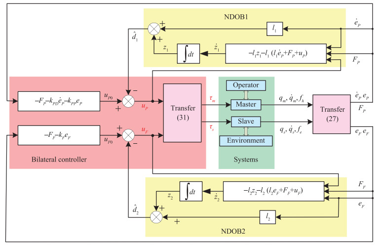
To estimate the lumped disturbances in position and force tracking error dynamics (28) and (29), the NDOB which is proposed in [13] is introduced and designed as follows:
| NDOB1:{˙z1=−l1z1−l1(l1˙eP+FP+uP)ˆd1=z1+l1˙eP | (32) |
| NDOB2:{˙z2=−l2z2−l2(l2eF+FF+uF)ˆd2=z2+l2eF | (33) |
where z1, z2 are the internal states of observers, l1, l2 are the observer gains to be designed, and ˆd1, ˆd2 are the estimations of disturbances d1(t), d2(t), respectively.
The proposed bilateral controller is constructed via introducing the estimations of NDOBs (32) and (33) into the baseline controller (30) as follows:
| uP=−FP−kPD˙eP−kPPeP−ˆd1uF=−FF−kFeF−ˆd2 | (34) |
where ˆd1 and ˆd2 are the disturbance estimations given by NDOBs (32) and (33), kPD, kPP and kF are the controller parameters to be designed. The control structure of the proposed bilateral controller is shown in Fig. 4.
Assumption 1: The derivatives of disturbances d1(t) and d2(t) in position and force control dynamics (28) and (29) are bounded, i.e., |˙d1(t)|≤kd1 and |˙d2(t)|≤kd2, with kd1>0 and kd2>0.
Assumption 2: The disturbances d1(t) and d2(t) in position and force tracking error dynamics (28) and (29) are constants in their steady states, i.e., limt→∞˙d1(t)=limt→∞˙d2(t)=0.
Lemma 1 [22]: The following linear systems:
| ˙xx=AAxx+BBuu | (35) |
is asymptotically stable if AA is Hurwitz matrix and \boldsymbol{u} is bounded and satisfies \mathop{\lim }_{t\to\infty}\|{\pmb u}(t)\|_2=0.
Theorem 1: Suppose that the Assumptions 1 and 2 are satisfied for systems (28) and (29). Considering the position and force control systems (28) and (29) under the proposed controller (34), the position and force tracking errors converge to zero asymptotically if the controller parameters are designed as k_{PP}>0, k_{PD}>0, k_{F}>0 and the observer gains l_1, l_2 in (32) and (33) are designed as positive constants.
Proof: Substituting the proposed controller (34) into the tracking error dynamics (28) and (29) yields
| \begin{align} \ddot e_P=&-k_{PD}\dot e_P-k_{PP}e_P-(\hat d_1-d_1)\nonumber\\ \dot e_F=&-k_Fe_F-(\hat d_2-d_2). \end{align} | (36) |
Define the estimation errors of d_1(t) and d_2(t) as
| \begin{align} \label{eed} e_{d1}=\hat d_1(t)-d_1(t), ~~e_{d2}=\hat d_2(t)-d_2(t). \end{align} | (37) |
The estimation error dynamics can be obtained from (28), (32) and (29), (33) respectively as
| \begin{align} \label{ded} \dot e_{d1}=-l_1 e_{d1}-\dot d_{1}, ~~~\dot e_{d2}=-l_2 e_{d2}-\dot d_{2}. \end{align} | (38) |
With (37) in mind, combining (36) and (38) obtains
| \begin{align} {\dot{{\pmb w}}}_1={\pmb A}_P{\pmb w}_1+{\pmb D}_{w1}, ~~~{\dot{\pmb w}}_2={\pmb A}_F {\pmb w}_2+ {\pmb D}_{w2} \end{align} | (39) |
with
| \begin{align*} &{\pmb w}_1=[e_P~\dot e_P~e_{d1}]^T, ~~~{\pmb w}_2=[e_F~e_{d2}]^T\\ &{\pmb D}_{w1}=[0~0~\dot d_1(t)]^T, ~~~{\pmb D}_{w2}=[0~\dot d_2(t)]^T\\ &{\pmb A}_P=\left[ {\begin{array}{*{20}{c}} 0 & 1 &0\\ -k_{PP} & -k_{PD} &-1\\ 0 & 0 &-l_1 \end{array}} \right], ~~ {\pmb A}_F=\left[ {\begin{array}{*{20}{c}} -k_{F} & -1\\ {{0}} &-l_2 \end{array}} \right]. \end{align*} |
Since k_{PP}>0, k_{PD}>0, k_{F}>0 and l_1, l_2 are positive constants, it can be verified that {\pmb A}_P and {\pmb A}_F are Hurwitz matrices. Since Assumptions 1 and 2 are satisfied, {\pmb D}_{w1} and {\pmb D}_{w2} in (39) are bounded and satisfy \mathop{\lim}_{t\to\infty} \|{\pmb D}_{w1}(t)\|_2=0 and \mathop{\lim}_{t\to\infty}\|{\pmb D}_{w2}(t)\|_2=0. Based on Lemma 1, it concludes from (39) that e_P, e_F, e_{d1} and e_{d2} converge to zero asymptotically.
Theorem 2: Suppose that the Assumption 1 is satisfied for systems (28) and (29). The proposed controller (34) guarantees that the position and force tracking errors converge to a bounded region if the controller parameters are designed as k_{PP} > 0, k_{PD}>0, k_{F}>0 and the observer gains l_1, l_2 in (32) and (33) are designed as positive constants.
Proof: Since {\pmb A}_P and {\pmb A}_F in (39) are Hurwitz matrices, there exist positive definite matrices {\pmb P}_1, {\pmb P}_2, {\pmb Q}_1 and {\pmb Q}_2 which satisfy
| \begin{align} \label{p20} {\pmb A}_P^T{\pmb P}_1+{\pmb P}_1{\pmb A}_P=-{\pmb Q}_1, ~~{\pmb A}_F^T{\pmb P}_2+{\pmb P}_2{\pmb A}_F=-{\pmb Q}_2. \end{align} | (40) |
Let us choose a Lyapunov function in terms of {\pmb w}_1 as
| \begin{align} \label{p21} V_1={\pmb w}_1^T{\pmb P}_1{\pmb w}_1. \end{align} | (41) |
With (40) in mind, taking the derivative of V_1 along (39) yields
| \begin{align*} \dot V_1 =&-{\pmb w}_{1}^T{\pmb Q}_1{\pmb w}_{1}+2{\pmb w}_{1}^T{\pmb P}_1{\pmb D}_{w1}\\ \leq& -\lambda_{\min}({\pmb Q}_1)\|{\pmb w}_{1}\|_2^2 +2\lambda_{\max}({\pmb P}_1)\|{\pmb w}_{1}\|_2 \cdot \|{\pmb D}_{w1}\|_2 \end{align*} |
where \lambda_{\min}({\pmb Q}_1) is the minimum eigenvalue of {\pmb Q}_1 and \lambda_{\max}({\pmb P}_1) is the maximum eigenvalue of {\pmb P}_1. With Assumption 1 in mind, it obtains from above equation that
| \begin{align} \dot V_1 \leq& -\lambda_{\min}({\pmb Q}_1)\|{\pmb w}_{1}\|_2^2 +2\lambda_{\max}({\pmb P}_1)\|{\pmb w}_{1}\|_2k_{d1}\nonumber\\ =& -\left[\lambda_{\min}({\pmb Q}_1)\|{\pmb w}_{1}\|_2 -2\lambda_{\max}({\pmb P}_1)k_{d1}\right] \cdot \|{\pmb w}_{1}\|_2. \end{align} | (42) |
It obtains from (41) that
| \begin{align} \label{p23} {{V}}_1\leq \lambda_{\max}({\pmb P}_1)\|{\pmb w}_{1}\|_2^2 \Rightarrow \|{\pmb w}_{1}\|_2 \geq \frac{{{V}}_1^{\frac{1}{2}}}{\sqrt{\lambda_{\max}({\pmb P}_1)}}. \end{align} | (43) |
When \|{\pmb w}_{1}\|_2 > \frac{2\lambda_{\max}({\pmb P}_1)k_{d1}}{\lambda_{\min}({\pmb Q}_1)}, combining (42) and (43) yields
| \begin{align} \label{p24} \dot V_1\leq -\frac{\epsilon}{\sqrt{\lambda_{\max}({\pmb P}_1)}}{{V}}_1^{\frac{1}{2}} \end{align} | (44) |
where
| \begin{align*} \epsilon=\lambda_{\min}({\pmb Q}_1)\|{\pmb w}_{1}\|_2-2\lambda_{\max}({\pmb P}_1)k_{d1}>0. \end{align*} |
It concludes from (44) that V_1 converges asymptotically until \epsilon>0 is not satisfied. This means both the position tracking error {{e}}_{P} and the disturbance estimation error {{e}}_{d1} converge to the following bounded region
| \begin{align} \label{p25} {|e_{P}|\leq r_1, ~~~|e_{d1}|\leq r_1, ~~~ r_1=\frac{2\lambda_{\max}({\pmb P}_1)k_{d1}} {\lambda_{\min}({\pmb Q}_1)}.} \end{align} | (45) |
Similarly, we can prove the force tracking error {{e}}_{F} and the disturbance estimation error {{e}}_{d2} converge to the following bounded region
| \begin{align} \label{p26} { |e_{F}|\leq r_2, ~~~|e_{d2}|\leq r_2, ~~~ r_2=\frac{2\lambda_{\max}({\pmb P}_2)k_{d2}} {\lambda_{\min}({\pmb Q}_2)}.} \end{align} | (46) |
Remark 5: The proposed controller rejects the disturbances' influence in force tracking error dynamics through a feedforward compensation way which guarantees fast convergence rate. While the force tracking error dynamics under the OCC law, the DC law and the MSSMC law in (17), (23) and (26) couple with system states, their convergence is obtained through feedback regulation in a relatively slow way.
Remark 6: The bounds of convergence regions (45) and (46) are determined by the controller parameters, observer gains and the bounds of disturbances' derivatives. They will decrease if k_{PD}, k_{PP}, k_{F} in controller (34) or l_1, l_2 in NDOBs (32) and (33) increase. This indicates that the convergence region in Theorem 2 can be assigned to be smaller by choosing larger controller parameters or observer gains.
Simulations are carried out in this part to validate the effectiveness of the proposed controller. To demonstrate the merits of the proposed controller, two popular linear bilateral control methods (i.e., the OCC method [10] and the DC method [11]), and a typical modal space based nonlinear bilateral controller (i.e., the MSSMC law [14]) are also employed here for comparisons. Similar with the simulation scenarios setting in [10] and [11], master and slave robots are set to have the same dynamics and the steady-state states of positions and contact forces are set as constants in our first simulation case. The model parameters of teleoperation systems (1)-(4) in this case are given by Table Ⅰ and they are all expressed in international standard units. To demonstrate the robustness of the proposed method, a more challenging and practical simulation case where master and slave robots have different dynamics under different types of external disturbances is also studied. The simulation scenario in this case is given in Table Ⅱ.
| Parameters of local site | Parameters of remote site |
| m_m=5, g_m=1, l_m=0.5 | m_s=5, g_s=1, l_s=0.5 |
| c_m(q_m, \dot q_m)=-8q_m-20\dot q_m | c_s(q_s, \dot q_s)=-8q_m-20\dot q_m |
| q_m(0)=0, ~x_{m0}=0 | q_s(0)=0.02, ~x_{s0}=0.01 |
| f_h^r=1, b_h=200, k_h=100 | f_e^r=0, b_e=200, k_e=100 |
| d_m =0.5 | d_s =0.5 |
 DownLoad:
CSV
DownLoad:
CSV
| Parameters of local site | Parameters of remote site |
| m_m=5, g_m=2, l_m=0.5 | m_s=10, g_s=4, l_s=0.5 |
| c_m(q_m, \dot q_m)=-8q_m-20\dot q_m | c_s(q_s, \dot q_s)=-20q_m-40\dot q_m |
| q_m(0)=0, ~x_{m0}=0 | q_s(0)=0, ~x_{s0}=0 |
| f_h^r=50-50\cos(\pi t) | f_e^r=0 |
| b_h=200, k_h=5000 | b_e=500, k_e=20\, 000 |
| d_m =\begin{cases} 0, & t\leq2 \\ 2\sin(\pi t), &2 <t\leq4.5\\ 2, &t>4.5 \end{cases} | d_s=\begin{cases} 0, &t\leq2 \\ 5\sin(\pi t), &2 <t\leq4.5\\5, &t>4.5 \end{cases} |
DownLoad:
CSV
The position and force scaling constants in (7) are set as \alpha = 1, \beta=0.2.
The proposed composite nonlinear bilateral controller is designed as (32)-(34), the controller parameters are set as l_1 =100, l_2=100, k_{PD}=40, k_{PP}=400, k_F=20.
The OCC law is designed as (10), (13) and (14), and the controller parameters are designed as g_m=100, g_s=100, k_{PD} =40, k_{PP}=400, k_F=100.
The DC law is designed as (13), (20) and (21), and the controller parameters are designed as g_X=100, g_F=100, k_{PD} =40, k_{PP}=400, k_F=100.
The MSSMC law is designed as (13), (24) and (25), and the controller parameters are designed as \eta_X=100, \eta_F=100, k_{PD} =40, k_{PP}=400, k_F=20.
The simulation results in this case under the four methods are given by Fig. 5. To demonstrate the simulation results more clearly, the zoom-in figures of contact force responses, position and force tracking error responses are also given in Fig. 5.
As shown in Fig. 5(e), all the four methods guarantee that the position tracking error converges to zero asymptotically and the zoom-in figure clearly demonstrates that the convergence rate of the proposed controller is faster than other three methods.
Fig. 5(f) illustrates the force tracking error responses under the four methods when constant contact forces and external disturbances act on the systems. The force tracking error response under the OCC method only converges to a bounded region which verifies the statement in Remark 2. The force tracking error under other three methods converge to zero asymptotically. The zoom-in figure shows the proposed method has the fastest convergence and this verifies the conclusions given in Remark 5. As stated in Remarks 3 and 4, the DC method solves the coupling problem of OCC and guarantees the force tracking error converge to zero, and the MSSMC method has a better dynamic response (i.e., faster convergence rate) than the DC method.
Fig. 6 gives the response curves of teleoperation systems under the four controllers in simulation Case Ⅱ. Figs. 6(e) and 6(f) demonstrate the position and force tracking errors under the OCC law divergence, this validates the statement in Remark 2 that the couplings in OCC law may result in unstable control performance. Fig. 6(e) illustrates that both the MSSMC method and the DC method guarantee the position tracking errors converge to a bounded region. The zoom-in figure of Fig. 6(e) clearly shows the proposed controller guarantees the position tracking error converge to zero asymptotically when there are no external disturbances (in the first two seconds) or the constant external disturbances (i.e., t > 4.5) acting on the systems, and the position tracking error is guaranteed to converge to a bounded region when time-varying disturbance acts on the systems (i.e., 2 <t\leq4.5). This verifies the conclusion in Theorems 1 and 2.
As stated in Remarks 3 and 4, the force tracking error under the DC method and the MSSMC method in Fig. 6(f) cannot be driven to the desired equilibrium point since the steady-state states of systems in this simulation case are not constants. To better demonstrate the force tracking performance in the presence of different types of external disturbances, force tracking error response curves are zoomed in and the zoom-in figure is given in Fig. 6(f). The proposed controller guarantees the force tracking error converge to zero asymptotically in the presence of constant disturbance (i.e., t>4.5) and this conforms to Theorem 1. When time-varying disturbance acts on the systems (i.e., 2 <t\leq4.5), the proposed controller guarantees the force tracking error converge to a bounded region and this verifies the conclusion given in Theorem 2.
This paper has investigated the bilateral controller design problem for nonlinear teleoperation systems with external disturbances. The main contribution here is to design a new composite bilateral control method which fully considers the contact force dynamics and systems' nonlinear dynamics such that the force control task is achieved through the combination of nonlinear feedback regulation and disturbance feedfoward compensation. The nonlinear disturbance observer has been employed to estimate the disturbances in position and force tracking error dynamics. The proposed composite bilateral controller has been constructed by introducing the disturbance estimations to the nonlinear controller design. Both the position and force tracking errors have been guaranteed to converge asymptotically by the proposed controller. The simulation results of a nonlinear teleoperation systems have validated the effectiveness of the proposed method.
| [1] |
P. F. Hokayem and M. W. Spong, "Bilateral teleoperation: an historical survey, " Automatica, vol. 48, no. 12, pp. 2035-2057, 2006. http://d.old.wanfangdata.com.cn/NSTLQK/NSTL_QKJJ026987994/
|
| [2] |
J. Yan, X. Yang, C. Chen, and X. Guan, "Bilateral teleoperation of multiple agents with formation control, " IEEE/CAA J. Autom. Sinica, vol. 1, no. 2, pp. 141-148, Apr. 2014.
|
| [3] |
P. Xiong, X. Zhu, A. Song, L. Hu, X. Liu, and L. Feng, "A target grabbing strategy for telerobot based on improved stiffness display device, " IEEE/CAA J. Autom. Sinica, vol. 4, no. 4, pp. 661-667, Oct. 2017.
|
| [4] |
Z. Li, X. Cao, and N. Ding, "Adaptive fuzzy control for synchronization of nonlinear teleoperators with stochastic time-varying communication delays" IEEE Trans. Fuzzy Syst., vol. 19, no. 4, pp. 745-757, Aug. 2011.
|
| [5] |
Z. Li, Y. Xia, D. Wang, D. H. Zhai, C. Y. Sun, and X. Zhao, "Neural network-based control of networked trilateral teleoperation with geometrically unknown constraints, " IEEE Trans. Cybern., vol. 46, no. 5, pp. 1051-1064, May 2016.
|
| [6] |
D. A. Lawrence, "Stability and transparency in bilateral teleoperation, " IEEE Trans. Robot. Autom., vol. 9, no. 5, pp. 624-637, Oct. 1993.
|
| [7] |
N. Hogan "Impedance control: an approach to manipulation: Part Ⅱ-Implementation, " J. Dyn. Syst. Meas. Control Trans. ASME, vol. 107, pp. 8-16, Mar. 1985.
|
| [8] |
L. J. Love and W. J. Book, "Force reflecting teleoperation with adaptive impedance control, " IEEE Trans. Syst., Man, Cybern. B, Cybern., vol. 34, no. 1, pp. 159-165, Feb. 2004.
|
| [9] |
J. Yang, S. Li, and X. Yu, "Sliding-mode control for systems with mismatched uncertainties via a disturbance observer, " IEEE Trans. Ind. Electron., vol. 60, no. 1, pp. 160-169, Jan. 2013.
|
| [10] |
S. Sakaino, T. Sato, and K. Ohnishi, "Multi-DOF micro-macro bilateral controller using oblique coordinate control, " IEEE Trans. Ind. Informat., vol. 7, no. 3, pp. 446-454, Aug. 2011.
|
| [11] |
T. Nozaki, T. Mizoguchi, and K. Ohnishi, "Decoupling strategy for position and force control based on modal space disturbance observer, " IEEE Trans. Ind. Electron., vol. 61, no. 2, pp. 1022-1032, Feb. 2014.
|
| [12] |
K. Ohnishi, M. Shibata, and T. Murakami, "Motion control for advanced mechatronics, " IEEE/ASME Trans. Mechatronics, vol. 1, no. 1, pp. 56- 67, Mar. 1996.
|
| [13] |
W. H. Chen, D. J. Ballance, P. J. Gawthrop, and J. O'Reilly, "A nonlinear disturbance observer for robotic manipulators, " IEEE Trans. Ind. Electron., vol. 47, no. 4, pp. 932-938, Aug. 2000.
|
| [14] |
A. Hace and M. Franc, "Pseudo-sensorless high-performance bilateral teleoperation by sliding-mode control and FPGA, " IEEE/ASME Trans. Mechatron., vol. 19, no. 1, pp. 384-393, Feb. 2014.
|
| [15] |
X. Liu, R. Tao, and M. Tavakoli, "Adaptive control of uncertain nonlinear teleoperation systems, " Mechatronics, vol. 24, no. 1, pp. 66-78, 2014. Feb. 2014.
|
| [16] |
W. H. Chen, J. Yang, L. Guo, and S. Li, "Disturbance-observer-based control and related methods-An overview, " IEEE Trans. Ind. Electron., vol. 63, no. 2, pp. 1083-1095, Feb. 2016.
|
| [17] |
W. He, S. Zhang, and S. S. Ge, "Boundary output-feedback stabilization of a Timoshenko beam using disturbance observer, " IEEE Trans. Ind. Electron., vol. 60, no. 11, pp. 5186-5194, Nov. 2013.
|
| [18] |
W. He and S. S. Ge, "Vibration control of a nonuniform wind turbine tower via disturbance observer, " IEEE/ASME Trans. Mechatron., vol. 20, no. 1, pp. 237-244, Feb. 2015.
|
| [19] |
W. He, Z. Yan, C. Sun, and Y. Chen, "Adaptive neural network control of a flapping wing micro aerial vehicle with disturbance observer, " IEEE Trans. Cybern., vol. 47, no. 10, pp. 3452-3465, Oct. 2017.
|
| [20] |
M. Chen, P. Chen, and C. C. Lim, "Adaptive neural fault-tolerant control of a 3-DOF model helicopter system, " IEEE Trans. Syst. Man Cybern.-Syst., vol. 46, no. 2, pp. 260-270, Feb. 2016.
|
| [21] |
C. Mitsantisuk, S. Katsura, and K. Ohishi, "Force control of human-robot interaction using twin direct-drive motor system based on modal space design, " IEEE Trans. Ind. Electron., vol. 57, no. 4, pp. 1383- 1392, Aug. 2010.
|
| [22] |
S. Li, J. Yang, W. H. Chen, and X. Chen, "Generalized extended state observer based control for systems with mismatched uncertainties, " IEEE Trans. Ind. Electron., vol. 59, no. 12, pp. 4792-4802, Dec. 2012.
|
| [1] | Zheng Chen, Shizhao Zhou, Chong Shen, Litong Lyu, Junhui Zhang, Bin Yao. Observer-Based Adaptive Robust Precision Motion Control of a Multi-Joint Hydraulic Manipulator[J]. IEEE/CAA Journal of Automatica Sinica, 2024, 11(5): 1213-1226. doi: 10.1109/JAS.2024.124209 |
| [2] | Dan Zhang, Jiabin Hu, Jun Cheng, Zheng-Guang Wu, Huaicheng Yan. A Novel Disturbance Observer Based Fixed-Time Sliding Mode Control for Robotic Manipulators With Global Fast Convergence[J]. IEEE/CAA Journal of Automatica Sinica, 2024, 11(3): 661-672. doi: 10.1109/JAS.2023.123948 |
| [3] | Zhongcai Zhang, Guangren Duan. Stabilization Controller of An Extended Chained Nonholonomic System With Disturbance: An FAS Approach[J]. IEEE/CAA Journal of Automatica Sinica, 2024, 11(5): 1262-1273. doi: 10.1109/JAS.2023.124098 |
| [4] | Haoxiang Ma, Mou Chen, Qingxian Wu. Disturbance Observer-Based Safe Tracking Control for Unmanned Helicopters With Partial State Constraints and Disturbances[J]. IEEE/CAA Journal of Automatica Sinica, 2023, 10(11): 2056-2069. doi: 10.1109/JAS.2022.105938 |
| [5] | Lu Zhang, Jun Yang, Shihua Li. A Model-Based Unmatched Disturbance Rejection Control Approach for Speed Regulation of a Converter-Driven DC Motor Using Output-Feedback[J]. IEEE/CAA Journal of Automatica Sinica, 2022, 9(2): 365-376. doi: 10.1109/JAS.2021.1004213 |
| [6] | Jinfei Hu, Zheng Chen, Xin Ma, Han Lai, Bin Yao. A Telepresence-Guaranteed Control Scheme for Teleoperation Applications of Transferring Weight-Unknown Objects[J]. IEEE/CAA Journal of Automatica Sinica, 2022, 9(6): 1015-1025. doi: 10.1109/JAS.2022.105626 |
| [7] | Tongfu He, Zhong Wu. Iterative Learning Disturbance Observer Based Attitude Stabilization of Flexible Spacecraft Subject to Complex Disturbances and Measurement Noises[J]. IEEE/CAA Journal of Automatica Sinica, 2021, 8(9): 1576-1587. doi: 10.1109/JAS.2021.1003958 |
| [8] | Zhijia Zhao, Zhijie Liu. Finite-Time Convergence Disturbance Rejection Control for a Flexible Timoshenko Manipulator[J]. IEEE/CAA Journal of Automatica Sinica, 2021, 8(1): 157-168. doi: 10.1109/JAS.2020.1003378 |
| [9] | Tinghua Li, Qinghua Yang, Xiaowei Tu, Bin Ren. An Improved Torque Sensorless Speed Control Method for Electric Assisted Bicycle With Consideration of Coordinate Conversion[J]. IEEE/CAA Journal of Automatica Sinica, 2020, 7(6): 1575-1584. doi: 10.1109/JAS.2020.1003360 |
| [10] | Muhammad Usman Asad, Umar Farooq, Jason Gu, Ghulam Abbas, Rong Liu, Valentina E. Balas. A Composite State Convergence Scheme for Bilateral Teleoperation Systems[J]. IEEE/CAA Journal of Automatica Sinica, 2019, 6(5): 1166-1178. doi: 10.1109/JAS.2019.1911690 |
| [11] | Jiajun Wang. Speed-assigned Position Tracking Control of SRM With Adaptive Backstepping Control[J]. IEEE/CAA Journal of Automatica Sinica, 2018, 5(6): 1128-1135. doi: 10.1109/JAS.2016.7510019 |
| [12] | Mou Chen. Robust Tracking Control for Self-balancing Mobile Robots Using Disturbance Observer[J]. IEEE/CAA Journal of Automatica Sinica, 2017, 4(3): 458-465. doi: 10.1109/JAS.2017.7510544 |
| [13] | Songsong Cheng, Shengguo Wang, Yiheng Wei, Qing Liang, Yong Wang. Study on Four Disturbance Observers for FO-LTI Systems[J]. IEEE/CAA Journal of Automatica Sinica, 2016, 3(4): 442-450. |
| [14] | Lu Wang, Jianbo Su. Trajectory Tracking of Vertical Take-off and Landing Unmanned Aerial Vehicles Based on Disturbance Rejection Control[J]. IEEE/CAA Journal of Automatica Sinica, 2015, 2(1): 65-73. |
| [15] | Pei Jia, Fei Hao, Hao Yu. Function Observer Based Event-triggered Control for Linear Systems with Guaranteed L∞-Gain[J]. IEEE/CAA Journal of Automatica Sinica, 2015, 2(4): 394-402. |
| [16] | Chaoxu Mu, Qun Zong, Bailing Tian, Wei Xu. Continuous Sliding Mode Controller with Disturbance Observer for Hypersonic Vehicles[J]. IEEE/CAA Journal of Automatica Sinica, 2015, 2(1): 45-55. |
| [17] | Yanlong Zhou, Mou Chen, Changsheng Jiang. Robust Tracking Control of Uncertain MIMO Nonlinear Systems with Application to UAVs[J]. IEEE/CAA Journal of Automatica Sinica, 2015, 2(1): 25-32. |
| [18] | Lijiao Wang, Bin Meng. Distributed Force/Position Consensus Tracking of Networked Robotic Manipulators[J]. IEEE/CAA Journal of Automatica Sinica, 2014, 1(2): 180-186. |
| [19] | Wen Qin, Zhongxin Liu, Zengqiang Chen. Formation Control for Nonlinear Multi-agent Systems with Linear Extended State Observer[J]. IEEE/CAA Journal of Automatica Sinica, 2014, 1(2): 171-179. |
| [20] | Jing Yan, Xian Yang, Cailian Chen, Xiaoyuan Luo, Xinping Guan. Bilateral Teleoperation of Multiple Agents with Formation Control[J]. IEEE/CAA Journal of Automatica Sinica, 2014, 1(2): 141-148. |

Figures(6) / Tables(2)


Zhenhua Zhao, Jun Yang, Shihua Li and Wen-Hua Chen, "Composite Nonlinear Bilateral Control for Teleoperation Systems With External Disturbances," IEEE/CAA J. Autom. Sinica, vol. 6, no. 5, pp. 1220-1229, Sept. 2019. doi: 10.1109/JAS.2018.7511273
| Parameters of local site | Parameters of remote site |
| m_m=5, g_m=1, l_m=0.5 | m_s=5, g_s=1, l_s=0.5 |
| c_m(q_m, \dot q_m)=-8q_m-20\dot q_m | c_s(q_s, \dot q_s)=-8q_m-20\dot q_m |
| q_m(0)=0, ~x_{m0}=0 | q_s(0)=0.02, ~x_{s0}=0.01 |
| f_h^r=1, b_h=200, k_h=100 | f_e^r=0, b_e=200, k_e=100 |
| d_m =0.5 | d_s =0.5 |
DownLoad:
CSV
| Parameters of local site | Parameters of remote site |
| m_m=5, g_m=2, l_m=0.5 | m_s=10, g_s=4, l_s=0.5 |
| c_m(q_m, \dot q_m)=-8q_m-20\dot q_m | c_s(q_s, \dot q_s)=-20q_m-40\dot q_m |
| q_m(0)=0, ~x_{m0}=0 | q_s(0)=0, ~x_{s0}=0 |
| f_h^r=50-50\cos(\pi t) | f_e^r=0 |
| b_h=200, k_h=5000 | b_e=500, k_e=20\, 000 |
| d_m =\begin{cases} 0, & t\leq2 \\ 2\sin(\pi t), &2 <t\leq4.5\\ 2, &t>4.5 \end{cases} | d_s=\begin{cases} 0, &t\leq2 \\ 5\sin(\pi t), &2 <t\leq4.5\\5, &t>4.5 \end{cases} |
DownLoad:
CSV
| Parameters of local site | Parameters of remote site |
| m_m=5, g_m=1, l_m=0.5 | m_s=5, g_s=1, l_s=0.5 |
| c_m(q_m, \dot q_m)=-8q_m-20\dot q_m | c_s(q_s, \dot q_s)=-8q_m-20\dot q_m |
| q_m(0)=0, ~x_{m0}=0 | q_s(0)=0.02, ~x_{s0}=0.01 |
| f_h^r=1, b_h=200, k_h=100 | f_e^r=0, b_e=200, k_e=100 |
| d_m =0.5 | d_s =0.5 |
| Parameters of local site | Parameters of remote site |
| m_m=5, g_m=2, l_m=0.5 | m_s=10, g_s=4, l_s=0.5 |
| c_m(q_m, \dot q_m)=-8q_m-20\dot q_m | c_s(q_s, \dot q_s)=-20q_m-40\dot q_m |
| q_m(0)=0, ~x_{m0}=0 | q_s(0)=0, ~x_{s0}=0 |
| f_h^r=50-50\cos(\pi t) | f_e^r=0 |
| b_h=200, k_h=5000 | b_e=500, k_e=20\, 000 |
| d_m =\begin{cases} 0, & t\leq2 \\ 2\sin(\pi t), &2 <t\leq4.5\\ 2, &t>4.5 \end{cases} | d_s=\begin{cases} 0, &t\leq2 \\ 5\sin(\pi t), &2 <t\leq4.5\\5, &t>4.5 \end{cases} |
 DownLoad:

 DownLoad:


