

Figure
1.
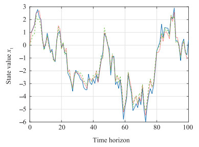
State trajectories of the first state component: real state value (solid line), its RHE estimation (dash-dotted line), and Kalman filter estimation (discontinuous line).
 Volume 6
Issue 2
Volume 6
Issue 2
IEEE/CAA Journal of Automatica Sinica
| Citation: | Chunyan Han, Chaochao Li, Fang He and Yue Liu, "Receding Horizon Estimation for Linear Discrete-time Systems with Multi-channel Observation Delays," IEEE/CAA J. Autom. Sinica, vol. 6, no. 2, pp. 478-484, Mar. 2019. doi: 10.1109/JAS.2018.7511261

|
At present, there are many methods to solve the state estimation problems of the discrete systems. Receding horizon estimation (RHE) or moving horizon estimation (MHE) is one of the most famous methods in the field of control and signal processing. RHE is an optimization-based state estimation technique which has received an increasing amount of attention in recent years. At each time, the current state estimate is determined by solving an optimization problem taking a number of past measurements into account. The advantage of the RHE is that it has good capacity to achieve rolling optimization and online application, and it has good robustness and stability. In practice, RHE can be applied widely to system state tracking, process monitoring, and equipment leak detection.
In recent years, a number of results have been reported about RHE. In [1], the problem of estimating the state of a dynamic system has been solved by introducing a receding horizon objective with a weighted penalty term, and a complete stability analysis has been explored. In [2], a receding horizon state observer, which used a deterministic least squares framework, was obtained. The state estimation horizon N was introduced as a tuning parameter for the proposed state observer, and a stability result concerning the choice of N was established. In addition, a robust receding-horizon estimation was addressed for a class of uncertain discrete-time linear systems in the presence of bounded uncertainty in [3]. For nonlinear systems, the receding horizon state estimation as well as the convergence problem were discussed in [4]-[6]. It was shown that one of the most advanced algorithms, which was especially applicable to nonlinear state estimation problem, was the moving horizon estimation [7]. In [8], the receding horizon estimator for nonlinear discrete-time systems affected by disturbances was designed according to a sliding-window strategy. In [9], a new receding-horizon nonlinear Kalman filter formulation for state estimation was proposed. It has been shown that the approach was able to handle constraints and provide immunity against poor initialization.
In [10], a new moving horizon estimator for nonlinear detectable systems was proposed, where the corresponding cost function contained an additional max term. The robust global asymptotic stability in case of bounded disturbances and convergence of the estimation error in case of vanishing disturbances were established. In [11], [12], the consensus-based distributed receding horizon estimation problems of sensor networked systems were discussed in detail. And, in [13], the basic design methods for ensuring stability of MHE were summarized and the relationships of full information and MHE to other state estimation methods such as Kalman filtering and statistical sampling were discussed. It can be found that seldom results have been reported for the receding horizon estimation subject to transmission delays.
There usually exist time delays in practical applications. For example, communication through band-limited linear filter channels may result in time delay phenomenon, and the low Earth orbit satellite communication systems usually have multiple channel delays. Because the presence of a time-delay often causes serious deterioration of the stability and performance of the system, considerable research has been devoted to the estimation of transmission delay systems [14]-[18] under different criteria and modeling methods. There exist several techniques for handling the delay terms, such as the classical state augmentation method [14], the polynomial approach [16], the linear matrix inequality algorithm [15], and the reorganization innovation analysis method [17], [18]. For linear systems with transmission time-delay, there also exist many papers proposing novel research in the literature. To handle time-varying communication delays, an open-loop state predictor was designed for each subsystem to provide predictions of unavailable subsystem states in [19]. In [20], a receding horizon filter for discrete-time linear system with uncertainties and time delays was proposed, where the filter gain was derived by solving a partial Riccati equation. In this paper, we will employ the tool of Riccati equation to derive the receding horizon estimation, which can reduce the calculation complexity for the design process.
This paper considers the receding horizon state estimation for the linear discrete-time system with multi-channel observation delays. The reorganized observation technique is employed for the design of the receding horizon estimation with time delays, and the filter gains are obtained by solving a set of Riccati equations. Two forms of the receding horizon estimation are developed, and the stability analysis is given. The main novelty of this paper is that we first apply the reorganized observation technique to solve the optimal receding horizon estimation subject to measurement delays. The proposed estimator has the same dimension as that of the original system, which reduces the computational burden greatly.
The remainder of this paper is organized as follows. The estimation problem statement for discrete-time linear systems is stated in Section Ⅱ. Section Ⅲ mainly concerns with the design of the receding horizon estimation and its stability analysis. In Section Ⅳ, attention is paid to a simulation example to evaluate the performance of the receding horizon estimation. Finally, conclusions are drawn in Section Ⅴ.
Consider the following discrete-time linear system with multi-channel observation delays:
| x(k+1)=Ax(k)+Cw(k),x(0)=x0 | (1) |
| yl(k)=Hlx(k−l)+vl(k−l),l=0,1,…,L | (2) |
where x(k)∈Rn is the state, w(k)∈Rr is the input noise, yl(k)∈Rpl is the measurement and vl(k)∈Rpl is the measurement noise. Throughout the paper, it is assumed that the constant matrices A, C, Hl are known, [C,A] is observable, A is nonsingular.
Assumption 1: w(k) and vl(k) are white noises with covariance matrices E{w(k)w(s)T}=Qδks, E{vl(k)vl(s)T}=Rlδks, respectively. x0, w(k), and vl(k) are mutually independent.
Denote
| y(k)={col{y0(k),…,yk(k),0,…,0},0≤k<Lcol{y0(k),…,yL(k)},k≥L |
then the optimal filtering problem considered in this paper can be stated as follows:
Optimal receding horizon estimation: Given the observation {y(s)|0≤s≤k}, find a linear minimum mean square error receding horizon estimator ˆx(k) of the state x(k) with the finite horizon N, such that Ew,v[ˆx(k)]=Ew,v[x(k)].
In this section, we will firstly introduce the observation reorganization technique to transform the measurement delay system into a delay-free one. Then, the receding horizon estimation with a batch form and an iterative form are structured, as well as the relevant proofs are given.
Since the multiple observation channels have different time delays, it is difficult to consider state estimation directly. All the observation channels need to be seen as a whole. Therefore, we can construct a new observation equation by the observation reorganization technique, which is without delay.
For the given time k, the received observations can be rearranged into a set of delay-free sequences as follows:
For 0≤s≤k−L,
| ˉyL(s)=[y0(s)⋮yL(s+L)]=[H0x(s)+v0(s)⋮HLx(s)+vL(s)]=[H0⋮HL]x(s)+[v0(s)⋮vL(s)]=ˉHLx(s)+ˉvL(s). | (3) |
For s=k−n (n=0,1,…,L−1)
| ˉyn(s)=[y0(s)⋮yn(s+n)]=[H0x(s)+v0(s)⋮Hnx(s)+vn(s)]=[H0⋮Hn]x(s)+[v0(s)⋮vn(s)]=ˉHnx(s)+ˉvn(s). | (4) |
The problem considered here is how to obtain a receding horizon estimate ˆx(k|k−1) of the state vector x(k) by using a finite number of measurements of the system output ˉy(k) with weighted matrix. A receding horizon estimation is derived from the following two theorems.
Theorem 1: For systems (1), (3) and (4), when (C,A) is observable, the receding horizon filter ˆx(k|k−1) with a batch form on the horizon [k−N,k] is derived by the following steps:
Step 1: For 0≤s≤k−L
| ˆx(s|s−1)=FLYL(s−1) | (5) |
where the optimal gain matrix FL is determined by
| FL=(ˉHTL,NΞ−1L,NˉHL,N)−1ˉHTL,NΞ−1L,N | (6) |
with
| YL(s−1)=[ˉyL(s−N)⋮ˉyL(s−1)] | (7) |
| ˉHL,N=[ˉHLA−N⋮ˉHLA−1] | (8) |
| ΞL,N=[ΞL,N−100RL,v]+[ˉHL,N−1ˉHL]×A−1CQwCTA−T[ˉHL,N−1ˉHL]TRL,v=diag{R1,R2,…,RL}. |
Step 2: For s=k−n;n=0,1,…,L−1
| ˆx(s|s−1)=FnYn(s−1) |
where the optimal estimate ˆx(k−n|k−n−1) is determined by the estimate of the time s=k−n−1, and the optimal gain matrix Fn is determined by
| Fn=(ˉHTn,NΞ−1n,NˉHn,N)−1ˉHTn,NΞ−1n,N |
with
| Yn(s−1)=[ˉyn(s−N)⋮ˉyn(s−1)]ˉHn,N=[ˉHnA−N⋮ˉHnA−1] |
| Ξn,N=[Ξn,N−100Rn,v]+[ˉHn,N−1ˉHn]×A−1CQwCTA−T[ˉHn,N−1ˉHn]TRn,v=diag{R1,R2,…,Rn}. |
Proof: For 0≤s≤k−L, the finite number of measurements on the horizon [s−N,s] can be expressed in terms of the state x(s)
| YL(s−1)=ˉHL,Nx(s)+ˉCL,NW(s−1)+ˉVL(s−1) | (9) |
where ˉHL,N is as in (8), and
| ˉCL,N=[ˉCL,N−1−ˉHL,N−1A−1C0−ˉHLA−1C] | (10) |
| W(s−1)=[w(s−N)⋮w(s−1)] | (11) |
| ˉVL(s−1)=[ˉvL(s−N)⋮ˉvL(s−1)] | (12) |
ˆx(s) can be indicated as a linear function of the finite measurements YL(s−1) on the horizon [s-N, s] as follows:
| ˆx(s|s−1)=FLYL(s−1)=FL(ˉHL,Nx(s)+ˉCL,NW(s−1)+ˉVL(s−1)) | (13) |
where
| FL=[FL,NFL,N−1…FL,1]. |
Taking the expectation on both sides of (13), the following relations are obtained
| Eˆx(s|s−1)=FLˉHL,NEx(s). |
To satisfy the unbiased condition, Eˆx=Ex, so
| FLˉHL,N=I. | (14) |
Deriving,
| ˆx(s|s−1)=x(s)+FLˉCL,NW(s−1)+FLˉVL(s−1). | (15) |
Thus, the estimation error can be represented as
| e(s)=ˆx(s|s−1)−x(s)=FLˉCL,NW(s−1)+FLˉVL(s−1). |
It can be shown that ˉCL,NW(s−1)+ˉVL(s−1) is with zero-mean and covariance matrix ΞL,N, which is given as
| ΞL,N=E[(ˉCL,NW(s−1)+ˉVL(s−1))(ˉCL,NW(s−1)+ˉVL(s−1))T]=ˉCL,NQNˉCTL,N+RL,N=[ˉCL,N−1QN−1ˉCTL,N−1+RL,N−100RL,v]+[ˉHL,N−1ˉHL]A−1CQwCTA−T[ˉHL,N−1ˉHL]T=[ΞL,N−100RL,v]+[ˉHL,N−1ˉHL]A−1×CQwCTA−T[ˉHL,N−1ˉHL]T | (16) |
where
| QN=diag{N⏞QwQw…Qw} |
| RL,N=diag{N⏞RL,vRL,v…RL,v}. |
The objective now is to obtain the optimal gain matrix FL, subject to the unbiasedness constraint (14), in such a way that the error e(s) of the estimate ˆx(s|s−1) has minimum variance as follows
| FL=argmin | (17) |
Before obtaining the solution to (16), we obtain the result on constraint optimization in the first place. To simplify the calculation, use \mathit{\boldsymbol{F}}_{L} as a temporary replacement of \mathit{\boldsymbol{F}}_{L}(s) . Now, suppose that the following trace optimization problem is given
| \begin{align} \min \limits_{\mathit{\boldsymbol{F}}}\{ {\rm{tr}} [(\mathit{\boldsymbol{F}}_{L}\bar{\mathit{\boldsymbol{C}}}_{L, N}) \mathit{\boldsymbol{Q}}_{N} (\mathit{\boldsymbol{F}}_{L}\bar{\mathit{\boldsymbol{C}}}_{L, N})^{T} + \mathit{\boldsymbol{F}}_{L}\mathit{\boldsymbol{R}}_{L, N}\mathit{\boldsymbol{F}}_{L}^{T}]\} \end{align} | (18) |
subject to
| \begin{eqnarray} \mathit{\boldsymbol{F}}_{L} {\bar{\mathcal{H}}}_{L, N} = \mathit{\boldsymbol{I}}. \end{eqnarray} | (19) |
For convenience, partition the matrix \mathit{\boldsymbol{F}}_{L} in (18) as
| \mathit{\boldsymbol{F}}_{L}^{T} = \left[ \begin{array}{ccccc} \mathit{\boldsymbol{f}}_{L, 1} & \ldots & \mathit{\boldsymbol{f}}_{L, j} & \ldots& \mathit{\boldsymbol{f}}_{L, N}\end{array} \right]. |
From (18), the s -th unbiasedness constraint can be written as
| \begin{eqnarray} {\bar{\mathcal{H}}}_{L, N}^{T}\mathit{\boldsymbol{f}}_{L, j} = \mathit{\boldsymbol{i}}_{j}. \end{eqnarray} | (20) |
In terms of the partitioned vector \mathit{\boldsymbol{f}}_{j} , the cost function (17) is represented as
| \begin{eqnarray} \sum\limits_{j = 1}^{N}\ [(\mathit{\boldsymbol{f}}_{L, j}^{T}\bar{\mathit{\boldsymbol{C}}}_{L, N}) \mathit{\boldsymbol{Q}}_{N} (\mathit{\boldsymbol{f}}_{L, j}^{T}\bar{\mathit{\boldsymbol{C}}}_{L, N})^{T} + \mathit{\boldsymbol{f}}_{L, j}^{T}\mathit{\boldsymbol{R}}_{L, N}\mathit{\boldsymbol{f}}_{L, j}].\ \end{eqnarray} |
Thus, the optimization problem (17) is reduced to N independent optimization problems
| \begin{eqnarray} \min \limits_{\mathit{\boldsymbol{f}}_{L, j}} \{(\mathit{\boldsymbol{f}}_{L, j}^{T}\bar{\mathit{\boldsymbol{C}}}_{L, N}) \mathit{\boldsymbol{Q}}_{N} (\mathit{\boldsymbol{f}}_{L, j}^{T}\bar{\mathit{\boldsymbol{C}}}_{L, N})^{T} + \mathit{\boldsymbol{f}}_{L, j}^{T}\mathit{\boldsymbol{R}}_{L, N}\mathit{\boldsymbol{f}}_{L, j}\} \end{eqnarray} | (21) |
subject to
| \begin{eqnarray} {\bar{\mathcal{H}}}_{L, N}^{T}\mathit{\boldsymbol{f}}_{L, j} = \mathit{\boldsymbol{i}}_{j}. \end{eqnarray} | (22) |
Obtaining the solutions to each optimization problem (20) and putting them together, we can finally get the solution to (17).
By the way of solving the optimization problem (21), we can establish the cost function
| \begin{align} \boldsymbol{\Phi} = & (\mathit{\boldsymbol{f}}_{L, j}^{T}\bar{\mathit{\boldsymbol{C}}}_{L, N}) \mathit{\boldsymbol{Q}}_{N} (\mathit{\boldsymbol{f}}_{L, j}^{T}\bar{\mathit{\boldsymbol{C}}}_{L, N})^{T}+\mathit{\boldsymbol{f}}_{L, j}^{T} \\ &{\times} \mathit{\boldsymbol{R}}_{L, N}\mathit{\boldsymbol{f}}_{L, j}+ \boldsymbol{\lambda}_{j}^{T}({\bar{\mathcal{H}}}_{L, N}^{T}\mathit{\boldsymbol{f}}_{L, j}- \mathit{\boldsymbol{i}}_{j}) \end{align} |
where \boldsymbol{\lambda}_j is the s -th vector of a Lagrange multiplier, which is associated with the s -th unbiased constraint.
In order to minimize \boldsymbol{\Phi} , two necessary conditions
| \frac{\partial \boldsymbol{\Phi}}{\partial \mathit{\boldsymbol{f}}_{L, j}} = 0, \frac{\partial \boldsymbol{\Phi}}{\partial \boldsymbol{\lambda}_{(j)}} = 0 |
are satisfied, which give
| \begin{eqnarray} \mathit{\boldsymbol{f}}_{L, j} = -\frac{1}{2} \boldsymbol{\Xi}_{L, N}^{-1} {\bar{\mathcal{H}}}_{L, N} \boldsymbol{\lambda}_{j}. \end{eqnarray} | (23) |
Thus
| {\bar{\mathcal{H}}}_{L, N}^{T} \mathit{\boldsymbol{f}}_{L, j} = -\frac{1}{2} {\bar{\mathcal{H}}}_{L, N}^{T} \boldsymbol{\Xi}_{L, N}^{-1} {\bar{\mathcal{H}}}_{L, N} \boldsymbol{\lambda}_{j} = \mathit{\boldsymbol{i}}_{j} |
then
| \begin{eqnarray} \boldsymbol{\lambda}_{j} = -2({\bar{\mathcal{H}}}_{L, N}^{T} \boldsymbol{\Xi}_{L, N}^{-1} {\bar{\mathcal{H}}}_{L, N})^{-1} \mathit{\boldsymbol{i}}_{j}. \end{eqnarray} | (24) |
From (23) and (24), we have
| \mathit{\boldsymbol{f}}_{L, j} = \boldsymbol{\Xi}_{L, N}^{-1} {\bar{\mathcal{H}}}_{L, N} ({\bar{\mathcal{H}}}_{L, N}^{T} \boldsymbol{\Xi}_{L, N}^{-1} {\bar{\mathcal{H}}}_{L, N})^{-1}\mathit{\boldsymbol{i}}_{j} |
and
| \mathit{\boldsymbol{f}}_{L, j}^{T} = \mathit{\boldsymbol{i}}_{j}^{T}({\bar{\mathcal{H}}}_{L, N}^{T} \boldsymbol{\Xi}_{L, N}^{-1} {\bar{\mathcal{H}}}_{L, N})^{-1}{\bar{\mathcal{H}}}_{L, N}^{T} \boldsymbol{\Xi}_{L, N}^{-1}. |
So put the above equation together, we can obtain
| \begin{eqnarray} \mathit{\boldsymbol{F}}_{L} = ({\bar{\mathcal{H}}}_{L, N}^{T} \boldsymbol{\Xi}_{L, N}^{-1} {\bar{\mathcal{H}}}_{L, N})^{-1}{\bar{\mathcal{H}}}_{L, N}^{T} \boldsymbol{\Xi}_{L, N}^{-1}. \end{eqnarray} | (25) |
Substitute (25) into (13), we can reach the batch form of receding horizon estimation
| \begin{align} \hat{ \mathit{\boldsymbol{x}}}(s|s-1) = &({\bar{\mathcal{H}}}_{L, N}^{T} \boldsymbol{\Xi}_{L, N}^{-1} {\bar{\mathcal{H}}}_{L, N})^{-1} \\ &{\times} {\bar{\mathcal{H}}}_{L, N}^{T} \boldsymbol{\Xi}_{L, N}^{-1}\mathit{\boldsymbol{Y}}_{L}(s-1). \end{align} | (26) |
This completes the proof of Step 1. The solution of Step 2 is similar to the solution of Step 1.
The filter with a batch form is represented in an iterative form for computational advantage. So we can get Theorem 2 by Theorem 1.
Theorem 2: Assume that (\mathit{\boldsymbol{C}}, \mathit{\boldsymbol{A}}) is observable. Then, the receding horizon filter \hat{\mathit{\boldsymbol{x}}}(k) with an iterative form is given on the horizon [k-N, k] by the following steps
Step 1: For 0\leq s \leq k-L ,
| \begin{eqnarray} \hat{\mathit{\boldsymbol{x}}}(s) = \mathit{\boldsymbol{P}}_{L, N}^{-1}\check{\mathit{\boldsymbol{x}}}(s) \end{eqnarray} | (27) |
where
| \begin{align} \check{ \mathit{\boldsymbol{x}}}(s) = &\, [\mathit{\boldsymbol{I}}+ \mathit{\boldsymbol{A}}^{-T} ( \mathit{\boldsymbol{P}}_{L, N-1}+ \bar{\mathit{\boldsymbol{H}}}_{L}^{T} \mathit{\boldsymbol{R}}_{L, v}^{-1} \bar{\mathit{\boldsymbol{H}}}_{L})\mathit{\boldsymbol{A}}^{-1} \\ & {\times} \, \mathit{\boldsymbol{C}}\mathit{\boldsymbol{Q}}_{w}\mathit{\boldsymbol{C}}^{T}]^{-1}\mathit{\boldsymbol{A}}^{-T}[\check{\mathit{\boldsymbol{x}}}(s-1) \\ & + \bar{\mathit{\boldsymbol{H}}}_{L}^{T}\mathit{\boldsymbol{R}}_{L, v}^{-1} \bar{\mathit{\boldsymbol{y}}}_{L}(s-1)] \end{align} | (28) |
and \mathit{\boldsymbol{P}}_{L, N} can be obtained from
| \begin{align} \mathit{\boldsymbol{P}}_{L, m} = &[\mathit{\boldsymbol{I}}+ \mathit{\boldsymbol{A}}^{-T} ( \mathit{\boldsymbol{P}}_{L, m-1}+ \bar{\mathit{\boldsymbol{H}}}_{L}^{T} \mathit{\boldsymbol{R}}_{L, v}^{-1} \bar{\mathit{\boldsymbol{H}}}_{L}) \mathit{\boldsymbol{A}}^{-1} \\ &{\times} \, \mathit{\boldsymbol{C}} \mathit{\boldsymbol{Q}}_{w}\mathit{\boldsymbol{C}}^{T} ]^{-1}\mathit{\boldsymbol{A}}^{-T} ( \mathit{\boldsymbol{P}}_{L, m-1} \\ &+ \bar{\mathit{\boldsymbol{H}}}_{L}^{T} \mathit{\boldsymbol{R}}_{L, v}^{-1} \bar{\mathit{\boldsymbol{H}}}_{L}) \mathit{\boldsymbol{A}}^{-1}, 1\leq m\leq N \end{align} | (29) |
with \mathit{\boldsymbol{P}}_{L, 0} = {\pmb{\mathit 0}} .
Step 2: For s = k-n;n = 0, 1, \ldots, L-1
| \begin{eqnarray} \hat{\mathit{\boldsymbol{x}}}(s) = \mathit{\boldsymbol{P}}_{n, N}^{-1}\check{\mathit{\boldsymbol{x}}}(s) \end{eqnarray} |
where
| \begin{align} \check{ \mathit{\boldsymbol{x}}}(s) = &\, [\mathit{\boldsymbol{I}}+ \mathit{\boldsymbol{A}}^{-T} ( \mathit{\boldsymbol{P}}_{n, N-1}+ \bar{\mathit{\boldsymbol{H}}}_{n}^{T} \mathit{\boldsymbol{R}}_{n, v}^{-1} \bar{\mathit{\boldsymbol{H}}}_{n})\mathit{\boldsymbol{A}}^{-1} \\ &{\times} \mathit{\boldsymbol{C}}\mathit{\boldsymbol{Q}}_{w}\mathit{\boldsymbol{C}}^{T}]^{-1}\mathit{\boldsymbol{A}}^{-T}[\check{\mathit{\boldsymbol{x}}}(s-1) \\ & + \bar{\mathit{\boldsymbol{H}}}_{n}^{T}\mathit{\boldsymbol{R}}_{n, v}^{-1} \bar{\mathit{\boldsymbol{y}}}_{n}(s-1)] \end{align} | (30) |
and \mathit{\boldsymbol{P}}_{n, N} can be obtained from
| \begin{align} \mathit{\boldsymbol{P}}_{n, m} = &\, [\mathit{\boldsymbol{I}}+ \mathit{\boldsymbol{A}}^{-T} ( \mathit{\boldsymbol{P}}_{n, m-1}+ \bar{\mathit{\boldsymbol{H}}}_{n}^{T} \mathit{\boldsymbol{R}}_{n, v}^{-1} \bar{\mathit{\boldsymbol{H}}}_{n}) \mathit{\boldsymbol{A}}^{-1} \\ &{\times} \mathit{\boldsymbol{C}} \mathit{\boldsymbol{Q}}_{w}\mathit{\boldsymbol{C}}^{T} ]^{-1}\mathit{\boldsymbol{A}}^{-T} ( \mathit{\boldsymbol{P}}_{n, m-1} \\ &+ \bar{\mathit{\boldsymbol{H}}}_{n}^{T} \mathit{\boldsymbol{R}}_{n, v}^{-1} \bar{\mathit{\boldsymbol{H}}}_{n}) \mathit{\boldsymbol{A}}^{-1}, 1\leq m\leq N \end{align} | (31) |
with \mathit{\boldsymbol{P}}_{n, 0} = {\pmb{\mathit 0}} .
Proof: Firstly, for 0\leq s\leq k-L , define
| \mathit{\boldsymbol{P}}_{L, N} = {\bar{\mathcal{H}}}_{L, N}^{T} \boldsymbol{\Xi}_{L, N}^{-1} {\bar{\mathcal{H}}}_{L, N}. |
Then, it can be expressed by the following Riccati Equation
| \begin{align} \mathit{\boldsymbol{P}}_{L, N} = & {\bar{\mathcal{H}}}_{L, N}^{T} \boldsymbol{\Xi}_{L, N}^{-1}{\bar{\mathcal{H}}}_{L, N} \\ = & \, \mathit{\boldsymbol{A}}^{-T} \left[ \begin{array}{c} {\bar{\mathcal{H}}}_{L, N-1} \cr \bar{\mathit{\boldsymbol{H}}}_{L} \end{array} \right]^{T} \Big( \boldsymbol{\Delta}_{L, N-1} + \left[ \begin{array}{c} {\bar{\mathcal{H}}}_{L, N-1} \cr \bar{\mathit{\boldsymbol{H}}}_{L} \end{array} \right] \mathit{\boldsymbol{A}}^{-1} \\ & {\times} \, \mathit{\boldsymbol{C}} \mathit{\boldsymbol{Q}}_{w} \mathit{\boldsymbol{C}}^{T}\mathit{\boldsymbol{A}}^{-T} \left[ \begin{array}{c} {\bar{\mathcal{H}}}_{L, N-1} \cr \bar{\mathit{\boldsymbol{H}}}_{L} \end{array} \right]^{T} \Big)^{-1} \left[ \begin{array}{c} {\bar{\mathcal{H}}}_{L, N-1} \cr \bar{\mathit{\boldsymbol{H}}}_{L} \end{array} \right] \mathit{\boldsymbol{A}}^{-1} \\ = & \, \mathit{\boldsymbol{A}}^{-T} \! \left[ \begin{array}{c} {\bar{\mathcal{H}}}_{L, N-1} \cr \bar{\mathit{\boldsymbol{H}}}_{L} \end{array} \right]^{T} \! \Big(\boldsymbol{\Delta}_{L, N-1}^{-1} - \boldsymbol{\Delta}_{L, N-1}^{-1} \\ &{\times} \! \left[\begin{array}{c} {\bar{\mathcal{H}}}_{L, N-1} \cr \bar{\mathit{\boldsymbol{H}}}_{L} \end{array}\right] \!\mathit{\boldsymbol{A}}^{-1} \mathit{\boldsymbol{C}} \Big\{ \mathit{\boldsymbol{I}}+ \mathit{\boldsymbol{C}}^{T} \mathit{\boldsymbol{A}}^{-T} \left[\begin{array}{c} {\bar{\mathcal{H}}}_{L, N-1} \cr \bar{\mathit{\boldsymbol{H}}}_{L} \end{array}\right]^{T} \\ &{\times} \boldsymbol{\Delta}_{L, N-1}^{-1}\left[\begin{array}{c} {\bar{\mathcal{H}}}_{L, N-1} \cr \bar{\mathit{\boldsymbol{H}}}_{L} \end{array}\right] \mathit{\boldsymbol{A}}^{-1} \mathit{\boldsymbol{C}} \Big\}\mathit{\boldsymbol{C}}^{T} \mathit{\boldsymbol{A}}^{-T} \\ &{\times} \left[\begin{array}{c} {\bar{\mathcal{H}}}_{L, N-1} \cr \bar{\mathit{\boldsymbol{H}}}_{L} \end{array}\right]^{T} \boldsymbol{\Delta}_{L, N-1}^{-1}\Big)^{-1}\left[\begin{array}{c} {\bar{\mathcal{H}}}_{L, N-1} \cr \bar{\mathit{\boldsymbol{H}}}_{L} \end{array}\right] \mathit{\boldsymbol{A}}^{-1} \\ = & \, \Big( \mathit{\boldsymbol{I}}- \mathit{\boldsymbol{A}}^{-T} \! \left[\begin{array}{c} {\bar{\mathcal{H}}}_{L, N-1} \cr \bar{\mathit{\boldsymbol{H}}}_{L} \end{array}\right]^{T} \! \boldsymbol{\Delta}_{L, N-1}^{-1} \! \left[\begin{array}{c} {\bar{\mathcal{H}}}_{L, N-1} \cr \bar{\mathit{\boldsymbol{H}}}_{L} \end{array}\right] \! \\ &{\times} \, \mathit{\boldsymbol{A}}^{-1}\mathit{\boldsymbol{C}} \Big\{ \mathit{\boldsymbol{I}}+ \mathit{\boldsymbol{C}}^{T} \mathit{\boldsymbol{A}}^{-T} \! \left[\begin{array}{c} {\bar{\mathcal{H}}}_{L, N-1} \cr \bar{\mathit{\boldsymbol{H}}}_{L} \end{array}\right]^{T} \! \boldsymbol{\Delta}_{L, N-1}^{-1} \\ &{\times} \, \! \left[\begin{array}{c} {\bar{\mathcal{H}}}_{L, N-1} \cr \bar{\mathit{\boldsymbol{H}}}_{L} \end{array}\right] \! \mathit{\boldsymbol{A}}^{-1}\mathit{\boldsymbol{C}} \Big\}\mathit{\boldsymbol{C}}^{T}\Big) \mathit{\boldsymbol{A}}^{-T} \! \left[\begin{array}{c} {\bar{\mathcal{H}}}_{L, N-1} \cr \bar{\mathit{\boldsymbol{H}}}_{L} \end{array}\right]^{T} \! \\ &{\times} \boldsymbol{\Delta}_{L, N-1}^{-1} \left[\begin{array}{c} {\bar{\mathcal{H}}}_{L, N-1} \cr \bar{\mathit{\boldsymbol{H}}}_{L} \end{array}\right]\mathit{\boldsymbol{A}}^{-1} \\ = & \, ( \mathit{\boldsymbol{I}}- \mathit{\boldsymbol{A}}^{-T} ( \mathit{\boldsymbol{P}}_{L, N-1}+ \bar{\mathit{\boldsymbol{H}}}_{L}^{T} \mathit{\boldsymbol{R}}_{L, v}^{-1} \bar{\mathit{\boldsymbol{H}}}_{L}) \mathit{\boldsymbol{A}}^{-1} \\ &{\times} \mathit{\boldsymbol{C}}\{ \mathit{\boldsymbol{I}}+ \mathit{\boldsymbol{C}}^{T} \mathit{\boldsymbol{A}}^{-T} ( \mathit{\boldsymbol{P}}_{L, N-1}+ \bar{\mathit{\boldsymbol{H}}}_{L}^{T} \mathit{\boldsymbol{R}}_{L, v}^{-1} \bar{\mathit{\boldsymbol{H}}}_{L}) \\ &{\times} \mathit{\boldsymbol{A}}^{-1} \mathit{\boldsymbol{C}} \}\mathit{\boldsymbol{C}}^{T}) \mathit{\boldsymbol{A}}^{-T} ( \mathit{\boldsymbol{P}}_{L, N-1}+\bar{\mathit{\boldsymbol{H}}}_{L}^{T}{\times} \mathit{\boldsymbol{R}}_{L, v}^{-1} \bar{\mathit{\boldsymbol{H}}}_{L} ) \mathit{\boldsymbol{A}}^{-1} \\ = & \, [\mathit{\boldsymbol{I}}+ \mathit{\boldsymbol{A}}^{-T} ( \mathit{\boldsymbol{P}}_{L, N-1}+ \bar{\mathit{\boldsymbol{H}}}_{L}^{T} \mathit{\boldsymbol{R}}_{L, v}^{-1} \bar{\mathit{\boldsymbol{H}}}_{L}) \mathit{\boldsymbol{A}}^{-1} \\ &{\times} \mathit{\boldsymbol{C}} \mathit{\boldsymbol{Q}}_{w} \mathit{\boldsymbol{C}}^{T} ]^{-1}\mathit{\boldsymbol{A}}^{-T} ( \mathit{\boldsymbol{P}}_{L, N-1}+ \bar{\mathit{\boldsymbol{H}}}_{L}^{T} {\times} \mathit{\boldsymbol{R}}_{L, v}^{-1} \bar{\mathit{\boldsymbol{H}}}_{L}) \mathit{\boldsymbol{A}}^{-1} \end{align} | (32) |
where
| \begin{eqnarray} \boldsymbol{\Delta}_{L, N-1} = \left[ \begin{array}{cc} \boldsymbol{\Xi}_{L, N-1} & 0 \cr 0 & \mathit{\boldsymbol{R}}_{L, v} \end{array} \right]. \end{eqnarray} |
\mathit{\boldsymbol{P}}_{L, 0} = {\pmb{\mathit 0}} should be satisfied to obtain the above \mathit{\boldsymbol{P}}_{L, 1} in Riccati (30).
Similarly, it is available that
| \begin{align} {\bar{\mathcal{H}}}_{L, N}^{T}\boldsymbol{\Xi}_{L, N}^{-1} = &\, [\mathit{\boldsymbol{I}}+ \mathit{\boldsymbol{A}}^{-T} ( \mathit{\boldsymbol{P}}_{L, N-1}+ \bar{\mathit{\boldsymbol{H}}}_{L}^{T} \mathit{\boldsymbol{R}}_{L, v}^{-1} \\ &{\times}\, \bar{\mathit{\boldsymbol{H}}}_{L}) \mathit{\boldsymbol{A}}^{-1} \mathit{\boldsymbol{C}} \mathit{\boldsymbol{Q}}_{w}\mathit{\boldsymbol{C}}^{T} ]^{-1}\mathit{\boldsymbol{A}}^{-T} \\ &{\times} \left[ \begin{array}{c} {\bar{\mathcal{H}}}_{L, N-1} \cr \bar{\mathit{\boldsymbol{H}}}_{L} \end{array} \right]^{T} \left[ \begin{array}{cc} \boldsymbol{\Xi}_{L, N-1} & 0 \cr 0 & \mathit{\boldsymbol{R}}_{L, v} \end{array} \right]. \end{align} | (33) |
On the basis of Theorem 1, we have
| \begin{align} \hat{ \mathit{\boldsymbol{x}}}(s+1) = &({\bar{\mathcal{H}}}_{L, N}^{T} \boldsymbol{\Xi}_{L, N}^{-1} {\bar{\mathcal{H}}}_{L, N})^{-1} \\ \quad{\times}& {\bar{\mathcal{H}}}_{L, N}^{T} \boldsymbol{\Xi}_{L, N}^{-1}\mathit{\boldsymbol{Y}}_{L, N}(s) \end{align} | (34) |
where
| \begin{eqnarray} \mathit{\boldsymbol{Y}}_{L, N}(s) = \left[ \begin{array}{c}\bar{\mathit{\boldsymbol{y}}}_{L}(s-N+1) \cr \vdots \cr \bar{ \mathit{\boldsymbol{y}}}_{L}(s) \end{array} \right]. \end{eqnarray} | (35) |
Now, we suppose that
| \begin{align} \check{ \mathit{\boldsymbol{x}}}(s) = &\, {\bar{\mathcal{H}}}_{L, N}^{T} \boldsymbol{\Xi}_{L, N}^{-1}\mathit{\boldsymbol{Y}}_{L, N}(s). \end{align} | (36) |
From (33) and (34), we can reach
| \begin{align} \check{ \mathit{\boldsymbol{x}}}(s) = &\, {\bar{\mathcal{H}}}_{L, N}^{T} \boldsymbol{\Xi}_{L, N}^{-1}\left[ \begin{array}{c} {\mathit{\boldsymbol{Y}}}_{L, N}(s-2) \cr \bar{ \mathit{\boldsymbol{y}}}_{L}(s-1) \end{array} \right] \\ = &\, [\mathit{\boldsymbol{I}}+ \mathit{\boldsymbol{A}}^{-T} ( \mathit{\boldsymbol{P}}_{L, N-1}+ \bar{\mathit{\boldsymbol{H}}}_{L}^{T} \mathit{\boldsymbol{R}}_{L, v}^{-1} \bar{\mathit{\boldsymbol{H}}}_{L}) \mathit{\boldsymbol{A}}^{-1} \\ & {\times} \, \mathit{\boldsymbol{C}} \mathit{\boldsymbol{Q}}_{w} \mathit{\boldsymbol{C}}^{T} ]^{-1} \mathit{\boldsymbol{A}}^{-T}[\check{\mathit{\boldsymbol{x}}}(s-1) \\ & + \bar{\mathit{\boldsymbol{H}}}_{L}^{T}\mathit{\boldsymbol{R}}_{L,v}^{-1} \bar{\mathit{\boldsymbol{y}}}_{L}(s-1)] \end{align} | (37) |
where \check{\mathit{\boldsymbol{x}}}(s-N) = 0 should be satisfied to obtain the same \check{\mathit{\boldsymbol{x}}}(s-N+1) in Riccati (35). From (32) and (35), an iterative form for receding horizon estimation is derived.
| \hat{\mathit{\boldsymbol{x}}}(s) = \mathit{\boldsymbol{P}}_{L, N}^{-1}\check{\mathit{\boldsymbol{x}}}(s). |
We are able to get iterative form for receding horizon estimation of Step 2 according to Step 1.
Remark 1: In this paper, the reorganized observation technique is employed for the design of the receding horizon estimation with multi-channel observation delays. Compared with the general state augmentation method [21], the approach employed in this paper reduces the computational burden greatly since the filter developed in Theorem 2 has the same dimension as that of the original system. This advantage is more evident in the case of systems with large time delays and high dimensions.
Remark 2: Due to the regular horizon term N is introduced in the optimized estimation, RHE can turn full information estimation problem into regular horizon estimation problem. And RHE is obtained by directly solving an optimization problem with the unbiasedness or deadbeatness constraint. Based on data from only the recent finite past (receding horizon), evidence shows that the proposed algorithm developed in Theorem 2 is more robust against dynamic model uncertainties compared with Kalman filters [20].
The stability of the receding-horizon filter will be investigated below. According to (28) and (30), it can be found that if the filter for 0\leq s \leq k-L is stable, the filter for s = k-L+1 is also stable since it is given by a recurrence Riccati equation of the previous sub-observer. Following a similar reasoning, all sub-observers will be stable. Then the stability of the overall filter will be reached. Thus we just need to analyze the stability of the filter developed in (27) and (28). This needs to require consideration of the filter's transfer matrix. From Theorem 2, we define the transfer matrix for 0\leq s \leq k-L as
| \begin{align} \boldsymbol{\Omega}_{L, N} = & [\mathit{\boldsymbol{I}}+ \mathit{\boldsymbol{A}}^{-T} ( \mathit{\boldsymbol{P}}_{L, N-1}+ \bar{\mathit{\boldsymbol{H}}}_{L}^{T} \mathit{\boldsymbol{R}}_{L, v}^{-1} \bar{\mathit{\boldsymbol{H}}}_{L}) \mathit{\boldsymbol{A}}^{-1} \\ & {\times} \mathit{\boldsymbol{C}} \mathit{\boldsymbol{Q}}_{w} \mathit{\boldsymbol{C}}^{T} ]^{-1}\mathit{\boldsymbol{A}}^{-T}\mathit{\boldsymbol{P}}_{L, N-1}^{-1}. \end{align} |
Under the given assumption, the necessary and sufficient condition subject to the asymptotic stability of the proposed filter is that the transfer matrix \boldsymbol{\Omega}_{L, N} of the filter is a stable matrix. It means that all of its eigenvalues are located in the unit circle. The stability of the observer is ensured by the following theorem.
Theorem 3: If (\mathit{\boldsymbol{C}}, \mathit{\boldsymbol{A}}) is observable, \mathit{\boldsymbol{A}} nonsingular, then the matrix \boldsymbol{\Omega}_{L, N} has all its eigenvalues strictly within the unit circle for all finite {\rm{N}} \geq t-1 where t is the dimension of the state vector.
Proof: The proof process is similar to [2], and thus is omitted here.
Remark 3: Conditions for the stability of the proposed MHE are proposed for time-invariant systems. The advantage of this filter is that it is easy to implement since the filter gain can be computed off-line.
In this section, a simulation example with two channels is considered to illustrate the efficiency of the receding horizon estimation. A comparison to the Kalman filter is supplied in the simulation result. In this simulation, we set the time horizon T = 100 , the filter horizon size N = 5 , the time-delay d = 1 . The parameters of the system are as follows
| \mathit{\boldsymbol{A}} = \left[ \begin{array}{cc} 0.9 & 0 \cr 0 & 0.9 \end{array} \right], \quad\mathit{\boldsymbol{C}} = \left[ \begin{array}{c} 1 \cr 2 \end{array} \right] |
| \mathit{\boldsymbol{H}}_{0} = \left[ \begin{array}{cc} 1.6 & 0 \cr 0 & 1.8 \end{array} \right], \quad\mathit{\boldsymbol{H}}_{1} = \left[ \begin{array}{cc} 0.6 & 0 \cr 0 & 0.8 \end{array} \right] |
where \{\mathit{\boldsymbol{w}}(k)\}, \{\mathit{\boldsymbol{v}}_0(k)\} and \{\mathit{\boldsymbol{v}}_1(k)\} are mutually independent zero-mean Wiener processes with covariance matrices \mathit{\boldsymbol{Q}} = \mathit{\boldsymbol{I}}_2, \mathit{\boldsymbol{R}}_0 = \mathit{\boldsymbol{I}}_2, and \mathit{\boldsymbol{R}}_1 = \mathit{\boldsymbol{I}}_2 , respectively. The initial state \mathit{\boldsymbol{x}}(0) is a random variable with \mbox{E}(\mathit{\boldsymbol{x}}(0)) = 0 and \mbox{E}(\mathit{\boldsymbol{x}}(0)\mathit{\boldsymbol{x}}(0)') = I_2 . In the actual system we use \mathit{\boldsymbol{x}}(0) = [0\ 0]' for the simulation.
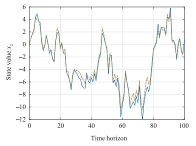
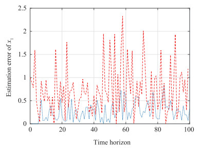
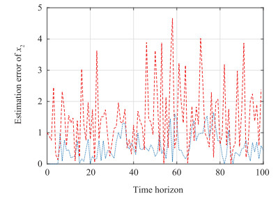
Following the design procedures as in Theorem 2 and Kalman filter, we obtain the simulation results as follows. Fig. 1 shows the trace of the real state value \mathit{\boldsymbol{x}}_{1}(k) and its estimate values according to the two algorithms. Fig. 2 shows the trace of the real state value \mathit{\boldsymbol{x}}_{2}(k) and its estimate values according to the two algorithms. Fig. 3 shows the root of mean square estimation errors of \mathit{\boldsymbol{x}}_{1}(k) according to the two algorithms, while Fig. 4 shows the root of mean square estimation errors of \mathit{\boldsymbol{x}}_{2}(k) according to the two algorithms. It can be seen from the simulation results that the obtained receding horizon estimation for systems with multiple-channel observation delays track better than Kalman filter and the estimation scheme proposed in this paper produces good performance.
In this note, we have studied the multi-channel receding horizon estimation for linear discrete-time system with observation delays. Firstly, the original multi-channel observation equations with time delays have been integrated by observation of reorganization. On the basis of observation of reorganization, a batch form and a recursive form for receding horizon estimation with some weighting gains were designed based on the measured data on the recent finite horizon [s-N, s] . And the stability of state estimation has been proven.
In this paper, the study mainly involves discrete linear systems. In fact, the solution to receding horizon problem for linear systems can be extended to infer receding horizon estimation of nonlinear systems. This work is worth researching further.
| [1] |
A. Alessandri, M. Baglietto, and G. Battistelli, "Receding-horizon estimation for discrete-time linear systems, " IEEE Trans. Autom. Control, vol. 48, no. 3, pp. 473-478, Mar. 2003. https://ieeexplore.ieee.org/document/1184901
|
| [2] |
K. V. Ling and K. W. Lim, "Receding horizon recursive state estimation, " IEEE Trans. Autom. Control, vol. 44, no. 9, pp. 1750-1753, Sep. 1999. https://www.researchgate.net/publication/3023479_Receding_Horizon_Recursive_State_Estimation
|
| [3] |
A. Alessandri, M. Baglietto, and G. Battistelli, "Robust receding-horizon estimation for discrete-time linear systems in the presence of bounded uncertainties, " in Proc. 44th IEEE Conf. Decision and Control, Seville, Spain, 2005, pp. 4269-4274. http://120.52.51.19/folk.ntnu.no/skoge/prost/proceedings/ecc03/pdfs/247.pdf
|
| [4] |
L. Ji, J. B. Rawlings, W. H. Hu, A. Wynn, and M. Diehl, "Robust stability of moving horizon estimation under bounded disturbances, " IEEE Trans. Autom. Control, vol. 61, no. 11, pp. 3509-3514, Nov. 2016. http://jbrwww.che.wisc.edu/tech-reports/twccc-2013-01.pdf
|
| [5] |
A. Wynn, M. Vukov, and M. Diehl, "Convergence guarantees for moving horizon estimation based on the real-time iteration scheme, " IEEE Trans. Autom. Control, vol. 59, no. 8, pp. 2215-2221, Aug. 2014. https://spiral.imperial.ac.uk/bitstream/10044/1/12628/2/MHE_Convergence.pdf
|
| [6] |
A. Alessandri, M. Baglietto, G. Battistelli, and T. Parisini, "New convergence conditions for receding-horizon state estimation of nonlinear discrete-time systems, " in Proc. 43rd IEEE Conf. Decision and Control, Nassau, Bahamas, 2004, pp. 2094-2099. https://ieeexplore.ieee.org/document/1430357
|
| [7] |
S. Kramer, R. Gesthuisen, and S. Engell, "Receding horizon state estimation with measurements at different sampling intervals, " in Proc. 2002 American Control Conf., Anchorage, AK, USA, 2002, pp. 905-906. https://wenku.baidu.com/view/78afb98d19e8b8f67c1cb98a.html
|
| [8] |
A. Alessandri, M. Baglietto, G. Battistelli, and T. Parisini, "Receding-horizon estimation for noisy nonlinear discrete-time systems, " in Proc. 42nd IEEE Conf. Decision and Control, Maui, Hawaii, USA, 2003, pp. 5825-5830. https://ieeexplore.ieee.org/document/1271934
|
| [9] |
R. Rengaswamy, S. Narasimhan, and V. Kuppuraj, "Receding-horizon nonlinear Kalman (RNK) filter for state estimation, " IEEE Trans. Autom. Control, vol. 58, no. 8, pp. 2054-2059, Aug. 2013. https://www.sciencedirect.com/science/article/pii/B9780444537119501693
|
| [10] |
M A Mddot{text{u}}ller, "Nonlinear moving horizon estimation in the presence of bounded disturbances, " Automatica, vol. 79, pp. 306-314, May 2017.
|
| [11] |
H. P. Li, W. S. Yan, and H. Z. Yang, "Receding horizon consensus estimation of sensor networks with packet dropouts, " in Proc. 34th Chinese Control Conf., Hangzhou, China, 2015, pp. 7659-7664.
|
| [12] |
H. P. Li and Y. Shi, "Consensus-based distributed receding horizon estimation of sensor networks, " in Proc. 32nd Chinese Control Conf., Xi'an, China, 2015, pp. 7483-7488.
|
| [13] |
J. B. Rawlings, Moving Horizon Estimation. London: Springer, 2014, pp. 1-7.
|
| [14] |
B. D. O. Anderson and J. B. Moore, Optimal Filtering. Englewood Cliffs, NJ: Prentice-Hall, 1979.
|
| [15] |
L. H. Xie, C. L. Du, C. S. Zhang, and Y. C. Soh, "H_{\infty} deconvolution filtering of 2-D digital systems, " IEEE Trans. Signal Process., vol. 50, no. 9, pp. 2319-2332, Sep. 2002.
|
| [16] |
L. Chisci, and E. Mosca, "Polynomial equations for the linear MMSE state estimation, " IEEE Trans. Autom. Control, vol. 37, no. 5, pp. 623-626, May 1992. https://www.researchgate.net/publication/266512049_Polynomial_MMSE_deconvolution_and_its_duality_with_LQGR
|
| [17] |
H. S. Zhang, L. H. Xie, D. Zhang, and Y. C. Soh, "A reorganized innovation approach to linear estimation, " IEEE Trans. Autom. Control, vol. 49, no. 10, pp. 1810-1814, Oct. 2004. A reorganized innovation approach to linear estimation
|
| [18] |
C. Y. Han, H. S. Zhang, and M. Y. Fu, "Optimal filtering for networked systems with markovian communication delays, " Automatica, vol. 49, no. 10, pp. 3097-3104, Oct. 2013. https://www.sciencedirect.com/science/article/pii/S000510981300366X
|
| [19] |
J. Zhang and J. F. Liu, "Observer-enhanced distributed moving horizon state estimation subject to communication delays, " J. Process Control, vol. 24, no. 5, pp. 672-686, May 2014.
|
| [20] |
I. Y. Song, D. Y. Kim, V. Shin, and M. Jeon, "Receding horizon filtering for discrete-time linear systems with state and observation delays, " IET Radar Sonar Navig., vol. 6, no. 4, pp. 263-271, Apr. 2012. https://www.researchgate.net/publication/235423662_Receding_Horizon_Filtering_for_Discrete-Time_Linear_Systems_with_State_and_Observation_Delays
|
| [21] |
Y. S. Lee and S. Han, "An improved receding horizon control for time-delay systems, " J. Optim. Theory Appl., vol. 165, no. 2, pp. 627-638, May 2015. doi: 10.1007/s10957-014-0658-8
|
| [1] | Bowen Sun, Xianghui Cao. Optimal Sensor Scheduling for Remote State Estimation With Partial Channel Observation[J]. IEEE/CAA Journal of Automatica Sinica. doi: 10.1109/JAS.2025.125180 |
| [2] | Shenquan Wang, Wenchengyu Ji, Yulian Jiang, Yanzheng Zhu, Jian Sun. Relaxed Stability Criteria for Time-Delay Systems: A Novel Quadratic Function Convex Approximation Approach[J]. IEEE/CAA Journal of Automatica Sinica, 2024, 11(4): 996-1006. doi: 10.1109/JAS.2023.123735 |
| [3] | Pengyan Huang, Guangchen Wang, Shujun Wang, Hua Xiao. A Mean-Field Game for a Forward-Backward Stochastic System With Partial Observation and Common Noise[J]. IEEE/CAA Journal of Automatica Sinica, 2024, 11(3): 746-759. doi: 10.1109/JAS.2023.124047 |
| [4] | Changjun He, Hua Geng, Kaushik Rajashekara, Ambrish Chandra. Analysis and Control of Frequency Stability in Low-Inertia Power Systems: A Review[J]. IEEE/CAA Journal of Automatica Sinica, 2024, 11(12): 2363-2383. doi: 10.1109/JAS.2024.125013 |
| [5] | Haotian Liu, Yuchuang Tong, Zhengtao Zhang. Human Observation-Inspired Universal Image Acquisition Paradigm Integrating Multi-Objective Motion Planning and Control for Robotics[J]. IEEE/CAA Journal of Automatica Sinica, 2024, 11(12): 2463-2475. doi: 10.1109/JAS.2024.124512 |
| [6] | Haihua Guo, Min Meng, Gang Feng. Lyapunov-Based Output Containment Control of Heterogeneous Multi-Agent Systems With Markovian Switching Topologies and Distributed Delays[J]. IEEE/CAA Journal of Automatica Sinica, 2023, 10(6): 1421-1433. doi: 10.1109/JAS.2023.123198 |
| [7] | PeiYun Zhang, MengChu Zhou, ChenXi Li, Abdullah Abusorrah. Dynamic Evolutionary Game-based Modeling, Analysis and Performance Enhancement of Blockchain Channels[J]. IEEE/CAA Journal of Automatica Sinica, 2023, 10(1): 188-202. doi: 10.1109/JAS.2022.105911 |
| [8] | Weiliang Zuo, Jingmin Xin, Changnong Liu, Nanning Zheng, Akira Sano. Improved Capon Estimator for High-Resolution DOA Estimation and Its Statistical Analysis[J]. IEEE/CAA Journal of Automatica Sinica, 2023, 10(8): 1716-1729. doi: 10.1109/JAS.2023.123549 |
| [9] | Mingming Ha, Ding Wang, Derong Liu. Discounted Iterative Adaptive Critic Designs With Novel Stability Analysis for Tracking Control[J]. IEEE/CAA Journal of Automatica Sinica, 2022, 9(7): 1262-1272. doi: 10.1109/JAS.2022.105692 |
| [10] | Xian-Ming Zhang, Qing-Long Han, Xiaohua Ge. Novel Stability Criteria for Linear Time-Delay Systems Using Lyapunov-Krasovskii Functionals With A Cubic Polynomial on Time-Varying Delay[J]. IEEE/CAA Journal of Automatica Sinica, 2021, 8(1): 77-85. doi: 10.1109/JAS.2020.1003111 |
| [11] | Pierluigi Di Franco, Giordano Scarciotti, Alessandro Astolfi. Stability of Nonlinear Differential-Algebraic Systems Via Additive Identity[J]. IEEE/CAA Journal of Automatica Sinica, 2020, 7(4): 929-941. doi: 10.1109/JAS.2020.1003219 |
| [12] | Jidong Wang, Zhanshan Wang, Sanbo Ding, Huaguang Zhang. Refined Jensen-Based Multiple Integral Inequality and Its Application to Stability of Time-Delay Systems[J]. IEEE/CAA Journal of Automatica Sinica, 2018, 5(3): 758-764. doi: 10.1109/JAS.2018.7511087 |
| [13] | Subir Das, Vijay K Yadav. Stability Analysis, Chaos Control of Fractional Order Vallis and El-Nino Systems and Their Synchronization[J]. IEEE/CAA Journal of Automatica Sinica, 2017, 4(1): 114-124. |
| [14] | Xiaojuan Chen, Jun Zhang, Tiedong Ma. Parameter Estimation and Topology Identification of Uncertain General Fractional-order Complex Dynamical Networks with Time Delay[J]. IEEE/CAA Journal of Automatica Sinica, 2016, 3(3): 295-303. |
| [15] | Xiaojun Tang, Jie Chen. Direct Trajectory Optimization and Costate Estimation of Infinite-horizon Optimal Control Problems Using Collocation at the Flipped Legendre-Gauss-Radau Points[J]. IEEE/CAA Journal of Automatica Sinica, 2016, 3(2): 174-183. |
| [16] | Xi Jin, Jintao Wang, Peng Zeng. End-to-end Delay Analysis for Mixed-criticality WirelessHART Networks[J]. IEEE/CAA Journal of Automatica Sinica, 2015, 2(3): 282-289. |
| [17] | Songmin Jia, Lijia Wang, Xiuzhi Li. View-invariant Gait Authentication Based on Silhouette Contours Analysis and View Estimation[J]. IEEE/CAA Journal of Automatica Sinica, 2015, 2(2): 226-232. |
| [18] | Wenhui Liu, Feiqi Deng, Jiarong Liang, Haijun Liu. Distributed Average Consensus in Multi-agent Networks with Limited Bandwidth and Time-delays[J]. IEEE/CAA Journal of Automatica Sinica, 2014, 1(2): 193-203. |
| [19] | Sen Wang, Ling Chen, Dongbing Gu, Huosheng Hu. Cooperative Localization of AUVs Using Moving Horizon Estimation[J]. IEEE/CAA Journal of Automatica Sinica, 2014, 1(1): 68-76. |
| [20] | Aolei Yang, Wasif Naeem, Minrui Fei. Decentralised Formation Control and Stability Analysis for Multi-vehicle Cooperative Manoeuvre[J]. IEEE/CAA Journal of Automatica Sinica, 2014, 1(1): 92-100. |

Figures(4)


Chunyan Han, Chaochao Li, Fang He and Yue Liu, "Receding Horizon Estimation for Linear Discrete-time Systems with Multi-channel Observation Delays," IEEE/CAA J. Autom. Sinica, vol. 6, no. 2, pp. 478-484, Mar. 2019. doi: 10.1109/JAS.2018.7511261
 DownLoad:

 DownLoad:


