On "Over-Sized" High-Gain Practical Observers for Nonlinear Systems

Ⅰ. INTRODUCTION

Aproblem found in several control and identification applications is the reconstruction of the unmeasurable state variables by the measures of the accessible ones [1]-[9]. This task has been extensively studied for both linear and nonlinear systems. For the formers, a rather standard solution is given by the Luenberger observer and the Kalman filter [10], [11]. On the other hand, when dealing with nonlinear systems, the problem of designing an observer is much more challenging. Many attempts have been made to provide a general framework that allows the structured design of observers. For instance, in [5], [12], [13], the observability problem is addressed by considering observers yielding error dynamics that, possibly after some coordinates transformation, become linear and spectrally assignable. Another technique that is widely used in industrial and manufacturing processes is the extended Kalman filter, whose design is based on a local linearization of the system around a reference trajectory [14]. A remarkable observer design technique has been proposed in [15], where Lyapunov-like conditions have been given for the existence of a nonlinear observer yielding asymptotically stable error dynamics (for more recent procedures allowing the structured design of observers, see [16], [17]).

The observer proposed in this paper belongs to the class of high-gain practical observers. Assuming that the system is in observability form and that the time derivatives of the output are bounded, such observers provide estimates of the state of the system yielding arbitrarily small estimation error with arbitrarily fast decay rate. The use of high-gains is a classical tool that has been extensively employed to compensate nonlinearities in the system: for instance in [18] a high-gain feedback stabilizing control algorithm is proposed for a class of nonlinear systems, in [19]-[22] it is shown how high-gain observers can be exploited to estimate the state of a nonlinear system, while in [23] it is shown how high-gain observers can be used in nonlinear feedback control.

The main objective of this paper is to show that, if the high-gain practical observer is designed to estimate the time derivatives of the output up to an order that is greater than the dimension of the state of the system (thus leading to the adjective over-sized), then the estimation error can be made smaller without increasing the gain. Thanks to their appealing properties (especially the fact that they do not require excessively large values of the observer gain), these observers have been already proved useful in several control and identification applications [24]-[28]. The performances of over-sized and normal-sized high-gain practical observers are compared by estimating the vertical velocity of an electron beam by measures collected at the Frascati Tokamak upgrade (FTU) facility.

Ⅱ. OBSERVABILITY FOR NONLINEAR SYSTEM

Consider the single-output, nonlinear system

where $f:\mathbb{R}\times \mathbb{R}^N\rightarrow\mathbb{R}^N$ and $h:\mathbb{R}^N\rightarrow \mathbb{R}^N$ are in $\mathcal{C}^k$ for some sufficiently large $k\in\mathbb{Z}$, $k>0$, $x(t)\in\mathbb{R}^N$ denotes the state of system (1), and $y(t)\in\mathbb{R}$ denotes its output. Let $\phi(t, x)$ denote the solution of system (1) at time $t\in\mathbb{R}$, $t\geq0$, starting at $x$, i.e., $\phi(0, x)=x$ for all $x\in\mathbb{R}^N$. Assume that $\phi(t, x)$ exists and is unique for all $t\in\mathbb{R}$, $t\geq0$, and $x\in\mathbb{R}^N$. System (1) is observable if any pair of different states $x, \xi\in\mathbb{R}^N$ is distinguishable, i.e., for each $x, \xi\in\mathbb{R}^N$, there exists $t\in\mathbb{R}$, $t\geq0$, such that $h(\phi(t, x))\neq h(\phi(t, \xi))$.

In this paper, single-output, (possibly, time varying) nonlinear systems that can be written in the following canonical observability form are considered:

$y_{e, N}=[\begin{array}{ccc} y_0&\cdots&y_N \end{array}]^{T}$, $\overline p:\mathbb{R}\times \mathbb{R}^{N+1}\rightarrow\mathbb{R}$ is $\mathcal{C}^k$ for some sufficiently large $k\in\mathbb{Z}$, $k>0$, and $y_{e, N}(t)$ is assumed to exist $\forall t\geq 0$. By construction, system (2) is observable [29].

The goal of this paper is to design an observer for system (2). Such a goal can be pursued by using classical high-gain practical observers (see, for instance, [20] and Section Ⅲ where the properties of such a class of observers are recalled). One of the main goals of this paper is to show that the performances of such observers can be improved by estimating, through another high-gain observer, more than $N$ time derivatives of the output (i.e., "oversizing" its state), without necessarily decreasing $\varepsilon$, as usual in high-gain observer design, that has several undesirable effects [4].

Ⅲ. NORMAL-SIZED HIGH-GAIN "PRACTICAL" OBSERVERS

In this section, some results about the standard normal-sized high-gain practical observers introduced in [20] are revised.

Let the polynomial $\lambda^{N+1}+\bar{\kappa}_1\lambda^N+\dots+\bar{\kappa}_N\lambda+\bar{\kappa}_{N+1}$ be Hurwitz and let $0 < \bar{\varepsilon}\ll1$ be a sufficiently small parameter. Under the assumptions of Theorems 2 and 3 of [20] (essentially, boundedness of $\bar{p}(t, y_{e, N}(t))$ as a function of $t$), a high-gain practical observer for (2) is given by

where $\hat{y}_{e, N}=[\begin{array}{ccc} \hat{y}_0 ~~~~ \cdots ~~~~ \hat{y}_N \end{array}]^{T}$ is an estimate of $y_{e, N}$.

Define the estimation error $\tilde{y}_{e, N}:=y_{e, N}-\hat{y}_{e, N}$, whose dynamics are given by

where

The following two lemmas and theorem, reported here for completeness, state that the output of the high-gain observer given in (3) is a practical estimate of the state of system (2).

Lemma 1 [20]: Let system (4) be given. There exists an $\bar{\varepsilon}$-dependent matrix $\bar{E}_{\bar{\varepsilon}}:= {\rm diag}~\{1, {\bar{\varepsilon}}, \dots, {\bar{\varepsilon}}^{N}\}$, such that

where

additionally, one has that

Lemma 2 [20]: Let $\Delta$ be the matrix defined in Lemma 1 and let $\bar{P}$ be the solution of the Lyapunov equation

Then, setting $\bar{P}_{\bar{\varepsilon}}=\bar{E}_{\bar{\varepsilon}}^{T} \bar{P} \bar{E}_{\bar{\varepsilon}}$, one has that

where $\bar{E}_{\bar{\varepsilon}}^{T} \bar{E}_{\bar{\varepsilon}}$ is a positive definite diagonal matrix.

Theorem 1 [20]: Consider the error dynamics given in (4). If there exists $\mu\in\mathbb{R}$, $\mu>0$, such that

where $\tilde{y}_{\bar{\varepsilon}} = \bar{E}_{\bar{\varepsilon}}\tilde{y}=\left[\begin{array}{cccc} \tilde{y}_1 & {\bar{\varepsilon}} \tilde{y}_2 & \cdots & {\bar{\varepsilon}}^{N}\tilde{y}_{N} \end{array}\right]^{T}$.

Ⅳ. OVER-SIZED HIGH-GAIN OBSERVERS

Consider now the following system:

where $\kappa_i$, $i=1, \dots, N+h$, are chosen so that the polynomial $\lambda^{N+h+1}+{\kappa}_1\lambda^{N+h}+\dots %+{\kappa}_{N+h}\lambda +{\kappa}_{N+h+1}$ is Hurwitz, $I_\ell$ denotes the $\ell$-dimensional identity matrix, $0_\ell$ denotes the $\ell$-dimensional zero matrix and $0 < {\varepsilon}\ll1$ is a sufficiently small parameter whose role is the same as of the parameter $\bar{\varepsilon}$ employed in (3).

The goal of this section is to show that the signal $\breve{y}_{e, N}$ is an estimate of the signal $y_{e, N}$ and that the $\mathcal{L}_2$ norm, over some suitably defined interval $\mathcal{I}$, of the estimation error $\check{y}_{e, N}=y_{e, N}-\breve{y}_{e, N}$ is lower than the one of $\tilde{y}_{e, N}$. By (2) and (7), the dynamics of the estimation error $\check{y}_{e, N}$ are given by

where

and $\xi_{N+1}$ is the output of the following linear system

where $C_3=[\begin{array}{ccccc} 1 & 0 & \cdots & 0 & 0 \end{array}]$, $\zeta(t)\in\mathbb{R}^{h}$, and

Hence, by defining $C_2:=[1 ~ 0 ~ \cdots ~ 0]$ and $\eta=\left[\check{y}_{e, N}^{T} ~ \zeta^{T} \right]^{T}$, one has that

where $\Lambda=\left[\begin{array}{c} B_2 \\ 0 \end{array}\right]$ and $\Theta=\left[\begin{array}{cc} A_2 &-B_2C_3\\ B_3C_2 & A_3 \end{array}\right]$.

The following two lemmas provide some properties of the matrices $\Theta$ and $\Lambda$ defining the dynamics of system (8).

Lemma 3: Let system (8) be given. There exists an $\varepsilon$-dependent matrix $E_\varepsilon:={\rm diag}\{1, \varepsilon, \dots, \varepsilon^{N+h}\}$, such that

where $\Phi := \left[\begin{array}{cc} \Phi_1 & \Phi_2\\ \Phi_3 & \Phi_4 \end{array}\right],$ $\Psi = \left[\begin{array}{c} B_2 \varepsilon^{N+1}\\ 0 \end{array}\right]$, with

Additionally, one has that

for all $\tau\geq 0$.

Proof: The expressions in (9) follow directly from the definition of the matrices $\Phi_i$, $i=1, \dots, 4$, and of the matrix $E_\varepsilon$. The expressions in (10) follows directly from the definition of the matrix exponential $\exp (A \tau ):=\sum_{k=1}^{\infty} A^k \frac{\tau^k}{k!}$.

Lemma 4: All the eigenvalues of the matrix $\Phi$ of (9), where $\bar{\kappa}_i$, $i=0, \dots, N+h+1$, are the coefficients given in (7), have negative real part.

Proof: By construction, $\Phi$ has the same characteristic polynomial of the companion matrix of the polynomial $\lambda^{N+h+1}+\bar{\kappa}_1\lambda^{N+h}+\dots+\bar{\kappa}_{N+h}\lambda+ \bar{\kappa}_{N+h+1}$, which is, by definition, Hurwitz. Hence, all the eigenvalues of the matrix $\Phi$ have negative real part.

Since, by Lemma 4, the matrix $\Phi$ is Hurwitz, then there exists a symmetric and positive definite solution $P$ to the Lyapunov equation [30]

Thus, letting $P_\varepsilon=E_\varepsilon^{T} P E_\varepsilon$, one has that

where $E_\varepsilon^{T} E_\varepsilon$ is a positive-definite diagonal matrix.

The following theorem and corollary state that $\breve{y}_{e, N}$ is a practical estimate of the signal $y_{e, N}$ (i.e., the error $\check{y}_{e, N}$ can be made arbitrarily small by choosing $\varepsilon$ sufficiently small).

Theorem 2: Consider the error dynamics given in (8). Let $P$ be the solution of the Lyapunov equation (11). If there exists a constant $\mu>0$ such that $\vert{\bar{p}(t, y_{e, N}(t))}\vert < \mu$, for all times $t\geq 0$, then there exists a time ${T}\geq 0$ such that

where $\eta_\varepsilon = E_\varepsilon\eta$.

Proof: Let $P_\varepsilon=E_\varepsilon^{T} P E_\varepsilon$. Consider the Lyapunov function

which is positive-definite, because the matrix $P_\varepsilon$ is positive-definite for all $\varepsilon$. Thus, computing the time derivative of $V(\eta)$ along the solutions of (8), one has that

Hence, by (12a), one has that

where $\eta_\varepsilon:=E_\varepsilon\eta$. Hence, under the assumption that $\vert{\bar{p}}\vert < \mu$, and by considering that $||{\Psi}||=\varepsilon^{N+1}$, then

Hence, for any $\eta_\varepsilon$ such that $||{\eta_\varepsilon}||>2 \mu \varepsilon^{N+1}||{P}||$, one has that $\dot{V} < 0$. Thus, since $V(\eta)=\eta^{T} P_\varepsilon \eta=\eta^{T} E_\varepsilon^{T} P E_\varepsilon \eta = \eta_\varepsilon^{T} P \eta_\varepsilon$, then $V(\eta)\leq||{\eta_\varepsilon}||^2||{P}||$. Thus, since $\dot{V}$ is negative definite for each $\eta_\varepsilon$ such that $||{\eta_\varepsilon}||>2\mu\varepsilon^{N+1}||{P}||$, there exists a time $T\geq t_0$, such that (13) holds [31].

Corollary 1: Let the assumptions of Theorem 2 hold. The estimation error $\check{y}_{e, N}(t)$ can be made arbitrarily small, for all times $t\geq T$, where $T$ is a sufficiently large time.

Proof: Let $V$ be the Lyapunov function used in the proof of Theorem 2. Consider that, by the definition of the vector $\eta_\varepsilon$,

where $\check{E}={\rm diag}\{1, \varepsilon, \dots, \varepsilon^{N}\}$. Since $E_{\varepsilon}$ is nonsingular, one has that $\eta_{\varepsilon}=0$ if and only if $\eta = 0$. Thus, by considering that, by (13), there is a sufficiently large $T$ such that

where $\underline{\lambda}=\lambda_{\rm min}{P}$, there exists a time $T$ such that $||{\check{y}_{e, N}(t)}||\leq 4\underline{\lambda}^{-1}\mu^2\varepsilon^{2N+2} ||{P}||^3, \forall t\geq T$. Therefore, the estimation error $\check{y}_{e, N}(t)$ can be made arbitrarily small, by decreasing $\varepsilon$.

In the remainder of this section, the estimates $\hat{y}_{e, N}$ and $\breve{y}_{e, N}$ of $y_{e, N}$ are compared. To carry out such a comparison, the following assumption is made.

Assumption 1: Let the coefficients $\bar{\kappa}_1, \dots, \bar{\kappa}_N$ and ${\kappa}_1, \dots, {\kappa}_{N+h}$ be chosen so that the matrices $\bar{P}$ and $P$, obtained by solving (5) and (11), respectively, are such that $||{P}||=||{\bar{P}}||,$ $\lambda_{\rm min}{P}=\lambda_{\rm min}{\bar{P}}$, and let $\bar{\varepsilon}=\varepsilon$.

Assumption 1 is made in order to guarantee that the "gain" of the high-gain observer given in (3) is the same "gain" of the high-gain observer given in (7). The following proposition and corollary show that the error $\check{y}_{e, N}$ obtained by using the over-sized observer (7) is lower than the error $\tilde{y}_{e, N}$, obtained by using the normal-sized observer (7), under Assumption 1.

Proposition 1: Let Assumption 1 hold, and let the assumptions of Theorems 1 and 2 hold. Let $\tilde{y}_{e, N}(t)$ be the state of system (4) at time $t$ and let $\check{y}_{e, N}(t)$ be the output of system (8) at time $t$, respectively. Then, there exists a sufficiently large time $T$, and a positive real constant $M$, such that $\check{y}_{e, N}(t)\leq M$ and $\tilde{y}_{e, N}(t)\leq M$, for all $t>T$.

Proof: Letting $\underline{\lambda}=\lambda_{\rm min}{P}=\lambda_{\rm min}{\bar{P}}$, by Theorem 1, one has that there exists a time $T_1$ such that $||{\tilde{y}_{\bar{\varepsilon}}(t)}||\leq 4\underline{\lambda}^{-1}\mu^2{\bar{\varepsilon}}^{2N+2}||{\bar{P}}||^3, \forall t\geq T_1$; on the other hand, by Theorem 2, there exists a time $T_2$ such that $||{\eta_\varepsilon(t)}||\leq 4\underline{\lambda}^{-1}\mu^2\varepsilon^{2N+2}||{P}||^3, \forall t\geq T_2$. Moreover, letting $\check{E}_{{\varepsilon}}$ be defined in (14), by Assumption 1, one has that $||{\check{E}_{{\varepsilon}}}||=||{E_{\bar{\varepsilon}}}||$. Hence, letting $T=\max\{T_1, T_2\}$, by considering that $||{\tilde{y}_{\bar{\varepsilon}}}|| = ||{E_{\bar{\varepsilon}} \tilde{y}_{e, N}}||$ and that, by the proof of Corollary 1, $||{\eta_\varepsilon}||\geq ||{\check{E}_\varepsilon \check{y}_{e, N}}||$, there exists a sufficiently large time $T$, and a positive real constant $M$, such that $||{\check{y}_{e, N}(t)}||\leq M$ and $||{\tilde{y}_{e, N}(t)}||\leq M$, $\forall t>T$.

Corollary 2: Let the assumptions of Proposition 1 hold. If, additionally, there does not exist a compact time interval $\mathcal{I}$ such that $\bar{p}(t, y_{e_N}(t))=0$, for almost all times $t \in \mathcal{I}$, then

for some $\delta_1>0$ and all $t\geq T$.

Proof: If there does not exist a time interval $\mathcal{I}$ such that $\bar{p}(t, y_{e_N}(t))=0$, $\forall t \in \mathcal{I}$, then by the dynamics of system (7), there does not exist a time interval $\mathcal{I}$, such that $y_0(t)=\xi_0(t)$, for all times $t\in\mathcal{I}$. Therefore, by (7d), there does not exist a time interval $\mathcal{I}$ such that $\xi_{N+h}(t)=0$, for all times $t\in\mathcal{I}$. Hence, by considering that $||{\eta_\varepsilon(t)}||=||{\check{E}_\varepsilon \check{y}_{e, N}}||+\delta(\zeta(t))$, where $\delta(\cdot)$ is a positive definite bounded function, and that there exists no time interval $\mathcal{I}$ such that $\zeta(t)=0$, for all times $t\in\mathcal{I}$, then, by the proof of Proposition 1, one has that

for all $t\geq T$. This proves the existence of a smaller upper-bound of the expression in the left-hand side of (15) with respect to normal-sized observers, suggesting that the over-sized observer achieves improved performance with respect to the index $\int_{\mathcal{I}}||{\check{y}_{e, N}}||^2(\tau)d\tau$, as also shown in Section Ⅵ.

Remark 1: Note that if $\bar p(t, y_{{e}, N})=\bar p(y_{{e}, N})$, $\bar p$ is linear with respect to $y_{e, N}$ and it is zero for some compact time interval $\mathcal{I}\triangleq [ \tau_1, \, \tau_2]$, $\tau_2>\tau_1\geq T$, then it vanishes identically for all $t \geq \tau_1$, since $y_{e, N}(t)$ is an analytic function of $t$. This would necessarily require that the observer implements an exact copy of the plant (null estimation error injection). In the case of normal-sized observer this implies that $\bar p(y_{{e}, N}(t))\equiv 0$, i.e., the plant is a pure chain of $N+1$ integrators (with no input). On the other hand, since we assumed that the over-sized observer has a state dimension larger than the plant, this contradicts the fact that the observer would implement a copy of the plant, and then such $\mathcal{I}$ cannot exist, yielding $\delta_1>0$ in (15).

Remark 2: The main advantage in the use of the over-sized observer (7) relies on the fact that, usually, high-gain practical observers yield estimates with larger errors in the higher order derivatives. Therefore, if one estimates time derivatives up to an order that is greater than the dimension of the system, the estimation error is gathered on the higher order derivatives (which are neglected for estimation purposes), thus leading to a smaller error in the estimation of the state of system (2), as confirmed theoretically by Proposition 1 and Corollary 2.

Ⅴ. THE LINEAR TIME-INVARIANT CASE

In this section, the filtering properties of the normal-sized and of the over-sized high-gain practical observers given in (3) and in (7), respectively, are discussed.

Consider the error dynamics given in (4) and (8). By considering $\bar {p}(t, y_{{e}, N}(t))$ as a time-dependent input function, systems (4) and (8) are linear and time-invariant, whence the transfer matrices, relating the input $\bar{p}(t):=\bar {p}(t, y_{{e}, N}(t))$ with $\tilde{y}_{e, N}$ and $\check{y}_{e, N}$, respectively, can be computed for such systems.

Consider the LTI system

The transfer matrix $H(s)$ of system (16) is given by $H(s)=C(sI-A)^{-1}B$. If the initial state of system (16) is $x(0)=0$, then, letting $u(s)=\mathscr{L}[u(t)]$, the Laplace transform $y(s)$ of the output $y(t)$ of system (16) is given by

Therefore, letting $\bar{p}(s)=\mathscr{L}[{\bar{p}(t)}]$, $\hat{C}_1=I_N$, $\hat{C}_2=[\begin{array}{cc} I_N & 0 \end{array}]$, and assuming that $\tilde{y}_{e, N}(0)=0$ and $\eta(0)=0$, the Laplace transform of the errors $\tilde{y}_{e, N}(t)$ and $\check{y}_{e, N}(t)$ can be obtained as

respectively. Given $A\in\mathbb{R}^{n\times n}$, $(sI-A)^{-1}$ can be computed by using the following Algorithm 1, where tr\, ($\cdot$) and det\, ($\cdot$) denote the trace and determinant operator, respectively.

By using such an algorithm, an explicit expression of the transfer matrices of systems (4) and (8) can be obtained.

Algorithm 1 [32]: Computation of the Matrix $(sI-A)^{-1}$
Input: A matrix $A\in \mathbb{R}^{n\times n}$.
Output: The matrix $(sI-A)^{-1}$.
1: Compute $d$ = det ($sI-A$).
2: Define $\alpha_n$ = 1 and $R_n = I$.
3: for $k=n-$1 to 0 do
4:Compute $\alpha_i$: = $(n-i)^{-1}$tr ($AR_{i+1}$).
5:Compute $R_i=\alpha_iI+AR_{i+1}$.
6: end for
7: Compute $(sI-A)^{-1}=d^{-1}\sum_{i=1}^{n}s^{i-1}R_i$.
8: return $(sI-A)^{-1}$.

 | Show Table

DownLoad: CSV

Lemma 5: Let systems (4) and (8) be given. Letting $\bar{\kappa}_0=\kappa_0=1$, the $\ell$th entry $[H_1(s)]_\ell$, $\ell=1, \dots, N+1$, of the transfer matrix $H_1(s)$ of system (4) is given by

whereas the $\ell$th entry $[H_2(s)]_\ell$, $\ell=1, \dots, N+1$, of the transfer matrix $H_2(s)$ of system (8) is given by

Proof: By using Algorithm 1, with $A_1\in\mathbb{R}^{(N+1)\times (N+1)}$ as input, to compute $(sI-A_1)^{-1}$, one has that $\alpha_{N}=\bar{\kappa}_1\bar{\varepsilon}^{-1}$ and $R_{N}=A_1+\bar{\kappa}_1\bar{\varepsilon}^{-1}I$. Assuming that, for a fixed $i$, $\alpha_{N+1-(i-1)}=\bar{\kappa}_{i-1}\bar{\varepsilon}^{-(i-1)}$ and that $R_{N+1-(i-1)}$ equals

then, by Steps 4 and 5 of Algorithm 1, $\alpha_{N+1-i}=\bar{\kappa}_{i}\bar{\varepsilon}^{i}$ and $R_{N+1-i}$ is given by the formula above, with $(i-1)$ substituted by $i$. Hence, by induction, the matrices $R_{N+1-i}$, $i=1, \dots, N$, are given by the expression above, with $(i-1)$ substituted by $i$. Therefore, letting $\bar{\kappa}_0:=1$, by (17a) and Step 7 of Algorithm 1 and by considering that det $(sI - A_1) = s^{N + 1} +$$\sum_{j=1}^{N+1}\frac{\bar{\kappa}_j}{\bar{\varepsilon}^j}s^{N+1-j}$, the $\ell$th entry $[H_1(s)]_\ell$, $\ell=1, \dots, N+1$, of the transfer matrix $H_1(s)$ of system (4) is given by

To prove that $[H_2(s)]_\ell$ is given by (19), define the matrix

which is trivially nonsingular. Consider now the matrix $\hat{\Theta}=T\Theta T^{-1}$. By using Algorithm 1, with input $\hat{\Theta}\in\mathbb{R}^ {(N+h+1)\times (N+h+1)}$, to compute $(sI-\hat{\Theta})^{-1}$, by the same reasoning of above, one has that the matrix $R_{N+h+1-i}$, $i=1, \dots, N+h$, of Algorithm 1 is given by

Therefore, by (17b) and by Step 7 of Algorithm 1 and by considering that det $(sI-\hat{\Theta})$ = det $(sI-\Theta)=s^{N+h+1}+ \sum_{j=1}^{N+h+1}\frac{\kappa_j}{\varepsilon^j} s^{N+h+1-j}$, and that $\hat{C}_2(sI-\Theta)^{-1}\Lambda=\hat{C}_2 T^{-1}{(sI-\hat{\Theta})^{-1}}T \Lambda$, the $\ell$th entry $[H_2(s)]_\ell$, $\ell=1, \dots, N+1$, of $H_2(s)$ is given by

where $\kappa_0=1$.

The transfer functions given in (18) and (19) can be used to wholly characterize the filtering properties of the observers given in (3) and (7).

Remark 3: The "extra" parameters in $H_2(s)$ can be tuned to make the amplitude of $H_2(s)$ smaller than $H_1(s)$, at least in some frequency range, while maintaining the same estimation error convergence (poles of $H_1(s)$ and $H_2(s)$ within a desired region). Therefore, the amplitude of the steady-state error induced by $\bar{p}(t)$ is reduced using over-sized observers.

The optimization could be performed either on the $\ell$th entry of the transfer function $H_2(s)$ or on the overall response to $\bar p(t)$, i.e., minimizing the $\mathcal{H}_2/\mathcal{H}_\infty$ norm of $H_2(s)$ with standard minimization tools (possibly scaled through a shaping function to allow a frequency dependent minimization).

Ⅵ. SIMULATION AND EXPERIMENTAL RESULTS

We now present two applications in which it is very important to provide the first derivative of the signals as accurate as possible. The first case is a numerical simulation by which we can show the improved performances of the proposed over-sized observer. Consider the second order LTI system

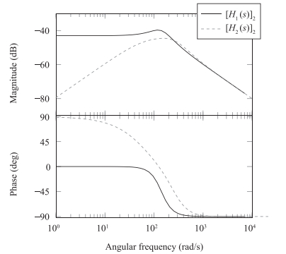
with $k=1.8$, $\lambda=1.8$, and $\omega_n=2\pi/0.16$. The transfer function $P(s)$ has been identified by experimental data in the Frascati Tokamak upgrade (FTU), a fusion reactor, in order to approximate the plasma current $I_p(s)\approx P(s)u(s)$ induced by the control input $u(t)$ (voltage to the central solenoid coil coupled with the plasma current, see [33] and [34] for further details). As in general plasma operation, the (normalized) input is picked as $u(t)=1-\exp(-t)$ to maintain a constant plasma current $I_p$. In the real plant the input $u(t)$ is provided by a standard PID regulator that is fed with the tracking error $I_{p, \rm reference}-I_p$ and its derivative $\dot I_{p, \rm reference}- \dot I_p$ (usually $\dot I_{p, \rm reference}=0$). The initial conditions of the plant are selected equal to $0$ for simplicity. The high-gain observers given in Sections Ⅲ and Ⅳ have been used to estimate $\dot y=\dot I_p$. In order to compare the two high-gain observers, a numerical constrained minimization has been carried out in order to determine $(\bar{\kappa}_1, \bar{\kappa}_2)\in[-500, 500]$ and $(\kappa_1, \kappa_2, \kappa_3)\in[-500, 500]$ such that, letting $N=1$, $h=1$, and $\varepsilon=\bar{\varepsilon}=0.05$, the $\mathcal{H}_2$ gain of the transfer functions $[H_1(s)]_{2}$ and $[H_2(s)]_{2}$ (given in (18) and (19), respectively), are minimized, while the roots of the polynomials $\lambda^{2}+\bar{\kappa}_1\lambda+\bar{\kappa}_2$ and $\lambda^{3}+{\kappa}_1\lambda^2+{\kappa}_2\lambda+\kappa_3$ have real part smaller than -2. The results of such minimizations are

that correspond to $\mathcal{H}_2$ gains $0.0841$ and $0.0633$, respectively. The Bode diagrams of the two optimized transfer functions of the high-gain observers are reported in Fig. 1: the $\mathcal{H}_2$ gain of the over-sized observer is lower than the normal one. In particular, for $\omega$ lower than $2\times 10^2$, one has $\vert H_1(\imath\, \omega) \vert < \vert H_2(\imath\, \omega)\vert$.

Figure  1.  Bode plots of $[H_1(s)]_2$ and $[H_2(s)]_2$.

DownLoad: Full-Size Img PowerPoint

These numerical computations corroborate the theoretical results given in this paper; in fact, they suggest again that, by allowing an "over-sizing" of the high-gain observer given in [20], improved performances can be achieved.

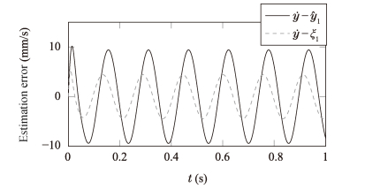
Fig. 2 depicts the results of such a numerical simulation by showing the difference between the analytical time derivative of the output $\dot y$ and its estimates obtained by using the normal-sized (with $N=1$) and over-sized (with $N=1$ and $h=1$) high-gain observers (3) and (7), respectively, where $\varepsilon=\bar{\varepsilon}=0.05$ and the $\bar{\kappa}_i$'s and $\kappa_j$'s are given in (20).

Figure  2.  Results of the numerical simulation.

DownLoad: Full-Size Img PowerPoint

The performances of the high-gain observer have improved by allowing its "over-sizing". As a matter of fact, one has that the estimation error resulting from the use of the over-sized high-gain practical observer is lower than the error obtained by employing the normal-sized one.

The two observers corresponding to the $\bar{\kappa}_i$'s and $\kappa_j$'s given in (20) and $\varepsilon=\bar{\varepsilon}=0.05$ have then been compared in a real experiment data. In this second case, we estimate the derivative of the runaway electron beams vertical position for which LTI models do not give satisfactory reconstruction, then we have only shown numerical results (in the previous case an analytic expression for $\dot y$ has been provided to compare the observers).

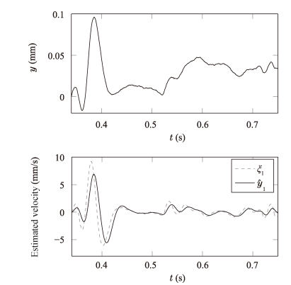
The measured plasma vertical position is first filtered with a first-order low-pass filter with cutoff frequency $100\, \mathit{\boldsymbol{Hz}}$ and is then fed to the normal-sized (with $N=1$) and over-sized (with $N=1$ and $h=1$) high-gain observers (3) and (7), where $\varepsilon=\bar{\varepsilon}=0.05$ and the $\bar{\kappa}_i$'s and $\kappa_j$'s are the ones given in (20). Fig. 3 depicts the filtered vertical position and the estimated velocities that have been obtained in such a numerical simulation. The over-sized high-gain observer seems to perform$^{1}$ better in estimating the derivative of the filtered signal $y$ (depicted in the same figure for completeness).

$^1$ In this case, since the analytical model is not available, only qualitative comparison can be achieved.

Figure  3.  Filtered position and estimated velocities: $\hat{y}_1$ has been obtained by using a normal-sized high-gain observer, whereas $\xi_1$ has been obtained by using an over-sized observer.

DownLoad: Full-Size Img PowerPoint

Note that the estimate of the vertical velocity, used by the feedback system to stabilize the runaway electron beam, is of crucial importance in order to avoid damages to the plant [35].

Ⅶ. CONCLUSIONS

In this paper, over-sized high-gain practical observers have been studied. It has been shown that, if one estimates the time derivatives of the output up to an order that is greater than the dimension of the system and takes into account just the first $N$ ones, then the estimation error decreases. The filtering properties of normal-sized and of the over-sized observers with respect to the unmodeled dynamics $\bar p (t)$ have been characterized by means of the corresponding transfer functions. Finally, the performances of the over-sized and normal-sized high-gain observers have been compared, analytically on an estimated model of the plasma current for FTU, and numerically for the estimation of the vertical velocity of a runaway electrons beam. It is worth noticing that such an over-sizing leads to an observer with an increased number of states and that the estimation error is fed back to the observer dynamics with (linear) gains that may be greater than the ones of the normal-sized observer. However, since such gains affect just the higher order dynamics of the observer, the undesirable effects of lowering the value of $\varepsilon$ are avoided.