

Figure
1.
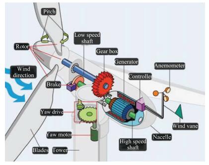
Wind turbine structure and major components (Figure courtesy of the U.S. Department of Energy [2]).
 Volume 4
Issue 3
Volume 4
Issue 3
IEEE/CAA Journal of Automatica Sinica
| Citation: | Wei Lin, Zongtao Lu and Wei Wei, "Asymptotic Tracking Control for Wind Turbines in Variable Speed Mode," IEEE/CAA J. Autom. Sinica, vol. 4, no. 3, pp. 569-576, July 2017. doi: 10.1109/JAS.2017.7510568

|
Renewable energy, especially wind energy, receives increasing attention over the past decade because of environmental concerns and pressures. Wind turbines, the electrical power generation plants from wind power, are structurally large and operating usually in harsh environments. How to efficiently control wind turbines is a challenging problem but of great significance for reducing the cost of wind energy.
Nowadays, most of the utility-scale turbines operate in variable speed mode. The speeds of wind turbines keep changing continuously in response to wind speed variation. The real-time adjustment of the turbine speed allows the wind turbine to operate longer at maximum aerodynamic efficiency, and hence capable of capturing more wind power than the constant speed operation. Additionally, variable speed turbines can filter out the generated power fluctuations and operating load changes that are caused by wind speed variation. Although variable speed wind turbines require complex and costly power electronics systems, the increasing efficiency provides enough benefit to compensate the cost and makes the required power electronics cost effective. As a result, the wind industry is inclined to design and build variable speed turbines [1]. On the other hand, the complex nature of the variable speed wind turbine system brings tremendous challenges, in particular, on how to effectively control variable speed turbines while reducing the cost of wind energy.
Fig. 1 shows a variable speed wind turbine structure and its major components. The wind comes across the rotor and causes it to spin. The low-speed shaft transfers the captured energy to the high speed shaft through the gearbox. The high speed shaft spins the generator and hence generates electricity. The yaw system is used to turn the nacelle so that the rotor faces directly into the wind.
A variable speed wind turbine has several levels of control systems. On the top level, a supervisory controller monitors the wind speed and direction to determine when the wind speed is sufficient to start up the turbine and when to shut down the wind turbine for safety due to too high wind speed. Typically, the operating modes of wind turbine are divided into three regions associated with wind speed, maximum allowable rotor speed and rated power. Fig. 2 shows a power curve versus wind speed for a wind turbine with three regions divided. Vcut−in is the {cut-in} wind speed at which the wind turbine starts to spin and Vcut−off is the wind speed at which the maximum allowable rotor speed is reached.
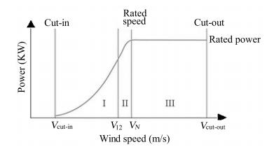
A wind turbine that is just starting up is considered to be operating in Region Ⅰ, i.e., the area from Vcut−in to V12 shown in Fig. 2. In Region Ⅱ (the area from V12 to VN of Fig. 2), the wind turbine is operating to maximize wind energy capture, which is realized by variable speed control with the pitch angle being usually kept constant. In Region Ⅲ ---the region ranges from VN to Vcut−off of Fig. 2, the turbine reaches and maintains its rated power PN. The captured power cannot be further increased even with higher speed wind, due to electrical and mechanical safety concerns of wind turbine systems.
The lower level of wind turbine control systems is turbine speed control, which includes generator torque control and blade pitch control. Generator torque control is to determine how much torque needs to be extracted from the turbine given the present wind speed. The extracted torque offsets the aerodynamic torque caused by the wind, and thus indirectly regulates the turbine speed. On the other hand, pitch control, manipulated by the pitch actuators, adjusts the pitch angle to the wind inflow and consequently regulates the turbine speed. In this paper, we focus on turbine control in Region Ⅱ, that is, the region from V12 to VN of Fig. 2, where pitch angle is usually kept constant and only torque control takes effect.
In the existing literature, there are some works that investigated modeling and control of variable speed wind turbine, such as [1], [3]-[10], just to name a few. Adaptive control design for wind turbines was studied in [3]. Based on the same model, a robust backstepping approach has been applied for the control system design [4]. Nonlinear power regulation for wind turbine was considered by [7]. Sliding mode and disturbance rejection controls were proposed in [6] and [10], respectively. The paper [5] developed a nonlinear control approach without wind speed measurement, yielding a robust nonlinear controller. More recently, the work [11] has developed a new maximum power point tracking (MPPT) algorithm for variable-speed wind turbine systems, by taking advantage of the rotor inertia power, while the paper [12] presented a MPPT algorithm that eradicates the problems that exist in the conventional hill-climbing MPPT technique. The proposed MPPT is a sensorless adaptive algorithm with higher control efficiency and faster tracking under rapid wind change. without requiring prior knowledge of the system's characteristics.
Wind turbines have been modeled as a one-mass drive-train system in several papers; see, for instance, [1], [5], and [6]. Although the one-mass drive-train model has a simple structure and is easy for the control design, it cannot capture the dynamics of torsional effects, which has a significant influence on the power fluctuations and the interaction of the wind turbine with the grid. Moreover, oversimplifying the models of wind turbine drive train could introduce significant error in dynamic behavior and stability [13]. Incorporating torsional effects, a linear system based on a two-mass drive-train model has been proposed in [9] for stability analysis. However, taking into account the aerodynamics, the wind turbine system is actually a nonlinear plant that is not in the so-called normal form [14]. This certainly raises a challenging issue on the design of nonlinear controllers for wind turbine systems described by a two-mass drive-train model, without linearizing the model.
In this paper, we present a geometric nonlinear control method to study the global tracking problem for variable speed wind turbines. The wind turbine is modeled as a two-mass drive-train system with generator torque control, which can be reduced to a one-mass drive-train system by assuming that the low speed shaft is perfectly rigid. Using the two-mass drive-train model, variable speed control schemes are investigated for Region Ⅱ. We design nonlinear tracking controllers to achieve global asymptotic tracking for a prescribed rotor speed reference signal so that maximum wind power capture can be yielded. Due to the difficulty of torsional angle measurement, we further develop an observer-based control scheme by using only the information of rotor speed to fulfill global asymptotic output tracking. Simulation results are given to illustrate the effectiveness of the proposed nonlinear control schemes.
The power extraction of wind turbine is a function of three main factors: the wind power available, the power curve of the machine and the ability of the machine to respond to wind fluctuation. As explained in [15] and [16], the available wind power is given by
| Pwind=12ρπR2wV3w | (1) |
and the power captured by the wind turbine is
| Pm=12Cp(λ,β)ρπR2wV3w | (2) |
where ρ is the air density, Rw is the blade tip radius, Vw is the wind speed and Cp is the power coefficient, which is a function of the tip-speed ratio λ and the pitch angle β. Note that the tip-speed ratio is defined as
| λ=RwωVw |
where ω is the rotor speed.
From the governing equation (2) for the generated power out of the wind turbine, it is clear that if the rotor speed is kept as a constant, a change in the wind speed will change the tip-speed ratio, leading to the changes of power coefficient Cp as well as the generated power out of the wind turbine. However, if the rotor speed is adjusted according to the wind speed variation, then the tip-speed ratio can be maintained at an optimal point, which could yield maximum power output from the system [3]. Consequently, we have the following relationship between captured wind power, rotor speed and rotor torque Ta,
| Pm(ω)=kwω3 | (3) |
| Ta=Pmω=kwω2 | (4) |
where
| kw=12CpρπR5wλ3. |
As shown in Fig. 3, the dynamics of wind turbine drive-train system can be modeled as a two-mass drive-train system. Driven by the aerodynamic torque Ta, the rotor of the wind turbine runs at the speed ω. The aeroturbine converts wind energy into mechanical energy, the gearbox serves to increase the speed ωg and decrease the torque from low speed shaft to the high speed shaft. The generator is to convert mechanical energy into electrical energy. Jr, Jg, Tls, Ths and Te denote rotor inertia, generator inertia, low speed shaft torque, high speed shaft torque and generator torque, respectively, br, bg, Cs and Ks are the damping and torsional coefficients.

The dynamics of the rotor is characterized by the first order differential equation
| Jr˙ω=Ta−Tls−brω. | (5) |
The low shaft speed results from the torsion and friction effects due to the difference between ω and ωls
| Tls=Ks(θ−θls)+Cs(ω−ωls). | (6) |
The generator is driven by the high speed shaft torque Ths and braked by the generator electromagnetic torque Te.
| Jg˙ωg=Ths−Te−bgωg. | (7) |
Through the gearbox, the low shaft speed ωls is increased by the gearbox ratio ng to obtain the generator speed ωg while the low speed shaft Tls torque is augmented.
| ng=TlsThs=ωgωls. | (8) |
Let θk=θ−θls. In view of the equations (4)-(8), the dynamics of the two-mass drive-train model can be represented by
| ˙θk=ω−1ngωg | (9) |
| ˙ω=1Jr(−Ksθk+kwω2−Csω−brω+Csngωg) | (10) |
| ˙ωg=1Jg(Ksngθk+Csngω−Csn2gωg−bgωg−Te). | (11) |
If a perfectly rigid low speed shaft is assumed, then ω=ωls. In this case, the two-mass drive-train model reduces to a one-mass drive-train model shown in Fig. 4. The governing dynamic equation is given by
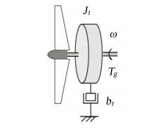
| Jt˙ω=Ta−btω−Tg | (12) |
where Jt=Jr+n2gJg, bt=br+n2gbg, Tg=ngTe.
Using (4), the dynamics of the one-mass drive-train model can be expressed as
| ˙ω=1Jt(−btω+kwω2−Tg). | (13) |
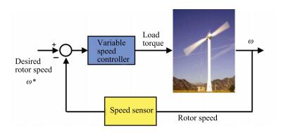
It is known that if the rotor speed is adjusted according to the wind speed variation, then the tip-speed ratio can be maintained at an optimal point, which could yield maximum power output from the system. A wind turbine control block diagram is shown in Fig. 5. The rotor speed of the wind turbine is controlled by the load torque. According to the feedback information of the current rotor speed, the control input Te is adjusted such that the rotor speed ω can track the desired rotor speed ω∗(t). Therefore, the tracking control problem in Region Ⅱ of Fig. 2 can be stated as follows. Design, if possible, a generator control torque Tg or Te such that the rotor speed ω of the wind turbine globally asymptotically tracks the desired speed ω∗(t). Throughout this work, it is assumed that ω∗(t), ˙ω∗(t) and ¨ω∗(t) are bounded.
For the two-mass drive-train model (9)-(11) of wind turbine system, the control objective is to force the output signal ω to track a prescribed reference signal ω∗(t). For the convenience of application of the geometric control method, the nonlinear system (9)-(11) can be transformed into a normal form [14] by introducing the change of coordinates
| z=θk | (14) |
| ξ1=ω | (15) |
| ξ2=−KsJrθk+CsJrngωg. | (16) |
Obviously, the transform above is a globally diffeomorphism. As a result, the nonlinear system in the new coordinates (z,ξ1,ξ2) is expressed as
| ˙z=−KsCsz+ξ1−JrCsξ2 | (17) |
| ˙ξ1=ξ2+ϕ1(ξ1) | (18) |
| ˙ξ2=v+ϕ2(z,ξ1,ξ2) | (19) |
| y=ξ1 | (20) |
where
| ϕ1(ξ1)=−Cs+brJrξ1+kwJrξ21ϕ2(z,ξ1,ξ2)=(K2sJrCs−bgKsJgJr)z+(C2sJrJgn2g−KsJr)ξ1+(KsCs−CsJgn2g−bgJg)ξ2v=−CsJgJrngTe |
the system output is ξ1=ω, ϕ1(ξ1) is a quadratic function of ξ1, and ϕ2(z,ξ1,ξ2) is linear with respect to z, ξ1 and ξ2.
Clearly, the nonlinear system (17)-(20) is minimum-phase because the zero dynamics ˙z=−(Ks/Cs)z is asymptotically stable. However, both the system output ξ1 and the state ξ2 drive the zero-dynamic system (17). This makes the global asymptotic tracking problem nontrivial. On the other hand, because the zero-dynamic system (17) is linear, it might be possible to utilize the idea of partial state feedback design [17] -[19], together with the tracking control strategy exploited in [20], to achieve global output tracking with stability. It turns out this idea works, as illustrated in the rest of this section.
To sum up, the wind turbine maximum power capture problem boils down to a global output tracking problem for the minimum-phase nonlinear system (17)-(20). The following condition characterizes what type of the reference signals can be tracked for variable speed wind turbines.
Assumption 1: A family of reference signals to be tracked, namely, yr(t)=ω∗(t), is assumed to be a bounded continuous function of time t with bounded first and second derivatives.
The first result of this paper is devoted to the global asymptotic tracking problem, illustrating how the problem can be solved by state feedback for the minimum-phase nonlinear system (17)-(20).
Theorem 1: Consider the equivalent wind turbine system (17)-(20). Given a prescribed reference speed signal ω∗(t) satisfying Assumption 1, there exists a state feedback controller v=β(z,ξ1,ξ2,yr,˙yr,¨yr), with β(0,0,0,yr,˙yr,¨yr)=0, such that the rotor speed ξ1=ω asymptotically tracks the desired speed yr(t)=ω∗(t), while maintaining global stability of the closed-loop system.
Proof: We begin with our proof by introducing the change of coordinates as done in [20]:
| e1=ξ1−yre2=ξ2−ξd2u=v−vd |
where ξd2=˙yr−ϕ1(yr), vd=˙ξd2−ϕ2(z,yr,ξd2).
Then, the nonlinear system (17)-(19) can be represented as
| ˙z=−KsCsz+e1−JrCse2+δ0(yr,˙yr) | (21) |
| ˙e1=e2+ˆϕ1(e1,yr) | (22) |
| ˙e2=u+ˆϕ2(e1,e2,yr,ξd2) | (23) |
where
| δ0(yr,˙yr)=yr−JrCsξd2ˆϕ1(e1,yr)=ϕ1(e1+yr)−ϕ1(yr)ˆϕ2(e1,e2,yr,ξd2)=ϕ2(z,e1+yr,e2+ξd2)−ϕ2(z,yr,ξd2) |
with ˆϕ1(0,yr)=0 and ˆϕ2(0,0,yr,ξd2)=0.
The asymptotic tracking control problem is to design a state feedback controller (using only the information of e1 and e2) for the nonlinear system (21)-(23) such that e1→0 as t tends to +∞, while maintaining global stability of the closed-loop system. Such a partial state feedback controller can be designed step by step by using the Lyapunov stability theory.
In the first step, consider the Lyapunov function
| V1(e1)=12e21. |
Taking a time derivative yields
| ˙V1=e1(e2+ˆϕ1(e1,yr))=−2e21+e1(e2−e∗2) |
where the virtual controller
| e∗2=2e1−ˆϕ1(e1,yr)=β1(e1,yr),β1(0,yr)=0. | (24) |
Next, consider the Lyapunov function
| V2=V1(e1)+12(e2−e∗2)2 |
whose time derivative along the system (22) and (23) satisfies
| ˙V2=−2e21+(e2−e∗2)[e1+u+ˆϕ2(⋅)−∂e∗2∂e1(e2+ˆϕ1(⋅))−∂e∗2∂yr˙yr]. |
Obviously, the partial state feedback controller
| u=−(e2−e∗2)−e1−ˆϕ2(⋅)+∂e∗2∂e1(e2+ˆϕ1(⋅))+∂e∗2∂yr˙yr= β2(e1,e2,yr,˙yr) | (25) |
with β2(0,0,yr,˙yr)=0 renders ˙V2 negative definite. In fact,
| ˙V2=−2e21−(e2−e∗2)2 |
which implies global asymptotic stability of (e1,e2)-subsystem of the nonlinear system (21)-(23).
Note that the zero dynamics ˙z=−(Ks/Cs)z of the nonlinear system (21)-(23) is asymptotically stable. In addition, the z-system (21) also satisfies the BIBO (bounded-input bounded output) property when viewing e1, e2 and δ0(yr,˙yr) as the system inputs. Consequently, the state z(t) is uniformly bounded ∀t, simply because (e1(t),e2(t))→0 as t tends to +∞ and δ0(yr,˙yr) is bounded. Thus, the nonlinear system (21)-(23) is globally stabilizable by the partial state feedback controller (25), with an asymptotic convergent property of the components (e1,e2). In particular,
| limt→+∞e1(t)=limt→+∞(ξ1(t)−yr(t))=0. |
In conclusion, the rotor speed of the wind turbine described by the two-mass drive-train model (17)-(19) can asymptotically track a prescribed speed yr(t)=ω∗(t) by the smooth state feedback controller
| v=u+vd=β2(e1,e2,yr,˙yr)+˙ξd2−ϕ2(z,yr,ξd2)=β(z,ξ1,ξ2,yr,˙yr,¨yr) | (26) |
with β(0,0,0,yr,˙yr,¨yr)=0.
The state feedback tracking controller (26) requires the information of all the system states, namely, θk, ω and ωg. However, the torsional angle θk is usually difficult to be measured in practice. For this reason, we propose an observer based control design, using ω and ωg information only, to achieve asymptotic tracking for a given reference speed signal yr(t) = ω∗(t).
Using the same change of coordinates (14)-(16) for the nonlinear system (9)-(11), we arrive at (17)-(20) in (z, ξ1, ξ2) coordinates. Note that ξ2 is not available for feedback design because it involves θk and the only measurable state is ξ1. Keeping this in mind, the problem boils down to the design of an output feedback tracking controller for the nonlinear system (17)-(20) by using ξ1 information only.
The following theorem is the main result of this work, showing how asymptotic tracking can be achieved by output feedback for the minimum-phase nonlinear system (17)-(20).
Theorem 2: Consider an equivalent wind turbine system (17)−(20). Given a prescribed reference speed signal ω∗(t) satisfying Assumption 1, there exists a smooth output feedback controller of the form
| ˙ς=Γ(ς,y),ς=[ˆzˆξ2]T | (27) |
| v=γ(y,ς,yr,˙yr,¨yr) | (28) |
with Γ(0,0)=0 and γ(0,0,yr,˙yr,¨yr)=0, such that the rotor speed y=ξ1=ω globally asymptotically follows the desired speed yr(t)=ω∗(t), while maintaining global stability of the closed-loop system.
Proof: This theorem can be proved by designing an output feedback controller with a reduced-order observer. Following the idea in [20], [21], we first construct a reduced-order observer to estimate the states z and ξ2. Due to the presence of the zero dynamics that were not considered in [20], the design of tracking controller here also involves the estimation of the state z of the zero-dynamics. Thanks to the linearity of the zero-dynamic equation (17) and the minimum-phase property, an output feedback tracking controller for the wind turbine system (17)-(20) can be constructed. For the convenience of the reader, we break up the design into two parts.
Part Ⅰ: Reduced-order Observer Design.
Consider the error dynamic system (21)-(23) in (z,e1,e2) coordinates. Introduce the rescaling transformation [20], [21]
| η1=e1andη2=e2M | (29) |
where M>0 is a gain constant to be determined later on.
In the (η1,η2) coordinate, (21)-(23) can be rewritten as
| ˙z=−KsCsz+η1−JrCsMη2+δ0(yr,˙yr) | (30) |
| ˙η1=Mη2+ˆϕ1(η1,yr) | (31) |
| ˙η2=uM+1Mˆϕ2(η1,η2,yr,˙yr). | (32) |
Define
| χ1=z−L1η1andχ2=η2−L2η1 |
where L1, L2>0 are constants to be determined later.
Naturally, the estimations of z and η2 can be given by
| ˆz=ˆχ1+L1η1andˆη2=ˆχ2+L2η1 |
where ˆχ1 and ˆχ2 are the estimations of χ1 and χ2, respectively, generated by the reduced-order observer
| ˙ˆχ1=−KsCsˆz+η1−JrCsMˆη2+δ0(⋅)−L1Mˆη2−L1ˆϕ1(η1,yr)˙ˆχ2= uM+1Mˆϕ2(η1,ˆη2,yr,˙yr)−L2Mˆη2−L2ˆϕ1(η1,yr). | (33) |
Introduce the estimate errors
| ε1=z−ˆz=χ1−ˆχ1andε2=η2−ˆη2=χ2−ˆχ2. |
Obviously, the errors satisfy the dynamic equation
| ˙ε1=−KsCsε1−(JrCs+L1)Mε2˙ε2=−L2Mε2+1M[ˆϕ2(η1,η2,yr,˙yr)−ˆϕ2(η1,ˆη2,yr,˙yr)]. | (34) |
Recall that the function ˆϕ2(⋅) is linear with respect to η1, η2, yr and ˙yr. Hence, it is easy to check that
| |ˆϕ2(η1,η2,yr,˙yr)−ˆϕ2(η1,ˆη2,yr,˙yr)|≤c|ε2| | (35) |
where c>0 is a known constant.
Consider the Lyapunov function
| V0(ε1,ε2)=12ε21+12ε22 |
whose time derivative satisfies
| ˙V0(ε1,ε2)=−KsCsε21−(JrCs+L1)Mε1ε2−L2Mε22+ε2M(ˆϕ2(η1,η2,yr,˙yr)−ˆϕ2(η1,ˆη2,yr,˙yr))≤−KsCsε21−(JrCs+L1)Mε1ε2−L2Mε22+cMε22. |
Choosing
| M=1, L1=1,andL2=1+c+(Jr+Cs)24KsCs |
results in
| ˙V0(ε1,ε2)≤−KsCs(ε1+Jr+Cs2Ksε2)2−ε22 | (36) |
which implies asymptotic stability of the error dynamics (34).
Part Ⅱ: Output Feedback Design.
To facilitate the design of an output tracking controller, we observe from (30)-(32) and (34) that the closed-loop system can be expressed as
| {˙ε1=−KsCsε1−(JrCs+L1)Mε2˙ε2=−L2Mε2+1M[ˆϕ2(η1,η2,yr,˙yr)−ˆϕ2(η1,ˆη2,yr,˙yr)]˙z=−KsCsz+η1−JrCsM(ˆη2+ε2)+δ0(yr,˙yr)˙η1=M(ˆη2+ε2)+ˆϕ1(η1,yr)˙ˆη2=uM+1Mˆϕ2(η1,ˆη2,yr,˙yr)+L2Mε2 | (37) |
with η1=e1 and ˆη2=ˆe2/M (in view of the rescaling transformation (29)).
Note that (η1,ˆη2)-subsystem of (37) can be represented in (e1,ˆe2)-coordinate as
| {˙e1=ˆe2+Mε2+ˆϕ1(e1,yr)˙ˆe2=u+ˆϕ2(e1,ˆe2,yr,˙yr)+L2M2ε2. | (38) |
For the system (38), consider the Lyapunov function
| W0(e1,ˆe2,yr)=12e21+12(ˆe2−e∗2)2 |
with W0(0,0,yr)=0, where e∗2 is given by (24).
A straightforward calculation shows that along the trajectories of (38), the time derivative of W0 satisfies
| ˙W0(e1,ˆe2,yr)= e1(−2e1+ˆe2−e∗2+Mε2)+(ˆe2−e∗2)[u+ˆϕ2(e1,ˆe2,yr,˙yr)+L2M2ε2−∂e∗2∂e1(e2+ˆϕ1(e1,yr))−∂e∗2∂yr˙yr]≤−e21+(ˆe2−e∗2)[e1+u+ˆϕ2(e1,ˆe2,yr,˙yr)−∂e∗2∂e1(ˆe2+Mε2+ˆϕ1(e1,yr))−∂e∗2∂yr˙yr+L2M2ε2]+M24ε22. |
Clearly, the implementable controller
| u=−(ˆe2−e∗2)−e1−ˆϕ2(e1,ˆe2,yr,˙yr)+∂e∗2∂yr˙yr+∂e∗2∂e1(ˆe2+ˆϕ1(e1,yr))−(ˆe2−e∗2)(L2M−∂e∗2∂e1)2= γ1(e1,ˆe2,yr,˙yr), with γ1(0,0,yr,˙yr)=0 | (39) |
is such that
| ˙W0(e1,ˆe2,yr)≤−e21−(ˆe2−e∗2)2+M22ε22. | (40) |
Now, consider the Lyapunov function
| W(ε1,ε2,e1,ˆe2,yr)=(1+M22)V0(ε1,ε2)+W0(e1,ˆe2,yr) |
for the closed-loop system (37).
In view of (36) and (40), it is easy to see that
| ˙W=(1+M22)˙V0+˙W0≤−KsCs(1+M22)(ε1+Jr+Cs2Ksε2)2−ε22−e21−(ˆe2−e∗2)2 |
which, in turn, implies asymptotic stability of ε-dynamics of (37) and (e1,ˆe2)-subsystem, and hence asymptotic stability of (e1,e2)-subsystem as well.
Finally, examine z-subsystem of the system (21). Obviously, the state z(t) remains uniformly bounded ∀t. This conclusion follows from the BIBO property of linear systems and the facts that δ0(yr,˙yr) is bounded and (e1(t),e2(t))→0 as t goes to +∞. In summary, the closed-loop system formed by (21)-(23), (33) and (39) is globally stable. Moreover, (e1,e2)-subsystem is asymptotically stable at (e1,e2)=(0,0). Therefore, asymptotic output tracking for the minimum-phase nonlinear system (17)-(19) can be achieved by an output feedback controller that is composed of the reduced-order observer (33) and the realizable controller (39) or, equivalently,
| v= u+vd= γ1(e1,ˆe2,yr,˙yr)+˙ξd2−ϕ2(ˆz,yr,ξd2)= γ(ξ1,ˆz,ˆξ2,yr,˙yr,¨yr) | (41) |
with γ(0,0,0,yr,˙yr,¨yr)=0.
By construction, the output feedback controller (33) and (41) is of the form (27) and (28).
Remark 1: For the closed-loop system represented by the (z,e)-coordinates and ε-dynamics, global asymptotic stability is only achieved for the (e,ε)-subsystem while global stability of the z-dynamics is obtained. In other words, the proposed output feedback control strategy ensures not only global asymptotic tracking for the output signal ξ1 of the wind turbine system, but also global stability of the closed-loop system.
So far it has been proved that a nonlinear state feedback controller and an observer-based output feedback controller can be designed for the two-mass drive-train model, globally asymptotically tracking a prescribed rotor speed reference signal as long as the signal to be tracked is bounded with bounded two-time derivatives. The proposed control scheme is applicable in Region Ⅱ of wind turbine operation (see Fig. 2), achieving the maximum wind power capture. The effectiveness of the tracking control scheme presented in this paper will be validated by simulations in the next subsection.
A simulation study is conducted to illustrate the proposed tracking control schemes. The wind turbine under study is with 1.7 MW rated power and the diameter of its blades is 35 meters [22]. The physical parameters are given in Table Ⅰ.
| Symbol | Value | Symbol | Value |
| Jr | 4×10⁶ kg⋅m2 | Jg | 20 kg⋅m2 |
| br | 980 N⋅m/s | bg | .2 N⋅m/s |
| ng | 38.06 | kw | 1.14×10⁵ kg⋅m2 |
| Ks | 10×6 N⋅m | Cs | 500 N⋅m/s |
 DownLoad:
CSV
DownLoad:
CSV
The rotor speed is required to track the desirable reference signal
| ω∗(t)=9.1+0.5(1+sin(π10t)). |
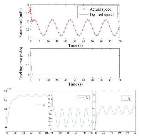
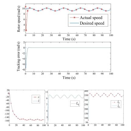
The simulation results with the state and output feedback controllers are shown in Figs. 6 and 7, respectively. It clearly demonstrates that the proposed control schemes are capable of achieving asymptotic tracking, while maintaining stability of the closed-loop system. As indicated in the simulation results, the settling time of the closed-loop system in the case of either state or output feedback is pretty short and reasonable, which is what we expect.
Variable speed control for wind turbine is necessary to increase the efficiency of wind power generation. In this paper, wind turbine system modeling and nonlinear tracking control have been investigated. A wind turbine is modeled as a two-mass drive-train system, which can be reduced to a one-mass drive-train model if the low speed shaft is assumed to be perfectly rigid. By introducing a suitable change of coordinates, the two-mass drive-train system can be transformed into a nonlinear system in a tractable form. By taking advantage of the minimum-phase property and the linearity of the zero-dynamic system of wind turbine, we have developed both state and output feedback tracking controllers that can achieve asymptotic tracking for the rotor speed with global stability. Analysis and simulations have indicated that the proposed methods are capable of achieving satisfactory rotor speed tracking, with global stability of the closed-loop system.
| [1] |
K. E. Johnson, L. Y. Pao, M. J. Balas, and L. J. Fingersh, "Control of variable-speed wind turbines: Standard and adaptive techniques for maximizing energy capture, " IEEE Control Syst. , vol. 26, no. 3, pp. 70-81, Jun. 2006. http://ieeexplore.ieee.org/xpls/icp.jsp?arnumber=1636311
|
| [2] |
U. S. Department of Energy. Energy efficiency and renewable energy, Technical Report. [Online]. Available: http://www.nrel.gov/docs/fy04osti/34915.pdf, Accessed on: Dec. , 2009.
|
| [3] |
Y. D. Song, B. Dhinakaran, and X. Y. Bao, "Variable speed control of wind turbines using nonlinear and adaptive algorithms, " J. Wind Eng. Industr. Aerodyn. , vol. 85, no. 3, pp. 293-308, Apr. 2000. http://www.sciencedirect.com/science/article/pii/S0167610599001312
|
| [4] |
S. Sivrioglu, U. Ozbay, and E. Zergeroglu, "Variable speed control of wind turbines:a robust backstepping approach, " in Proc. 17th IFAC World Congr., Seoul, Korea, 2008, pp. 1183-1188. https://www.researchgate.net/publication/267335504_Variable_Speed_Control_of_Wind_Turbines_A_Robust_Backstepping_Approach
|
| [5] |
B. Boukhezzar and H. Siguerdidjane, "Nonlinear control of variable speed wind turbines without wind speed measurement, " in Proc. 44th IEEE Conf. Decision and Control, Seville, Spain, 2005, pp. 3456-3461. http://ieeexplore.ieee.org/xpls/icp.jsp?arnumber=1582697
|
| [6] |
B. Beltran, T. Ahmed-Ali, and M. El Hachemi Benbouzid, "Sliding mode power control of variable-speed wind energy conversion systems, " IEEE Trans. Energy Convers. , vol. 23, no. 2, pp. 551-558, Jun. 2008. http://ieeexplore.ieee.org/document/4270775/
|
| [7] |
B. Boukhezzar and H. Siguerdidjane, "Nonlinear control of variable speed wind turbines for power regulation, " in Proc. 2005 IEEE Conf. Control Applications, Toronto, Canada, 2005, pp. 114-119. http://ieeexplore.ieee.org/xpls/icp.jsp?arnumber=1507110
|
| [8] |
L. Y. Pao and K. E. Johnson, "A tutorial on the dynamics and control of wind turbines and wind farms, " in Proc. 2009 American Control Conf., St. Louis, MO, USA, 2009, pp. 2076-2089. http://dl.acm.org/citation.cfm?id=1702657
|
| [9] |
C. Wang and G. Weiss, "Stability analysis of the drive-train of a wind turbine with quadratic torque control, " Int. J. Robust Nonlinear Control, vol. 19, no. 17, pp. 1886-1895, Nov. 2009. doi: 10.1002/rnc.1410/citedby
|
| [10] |
S. C. Thomsen and N. K. Poulsen, "A disturbance decoupling nonlinear control law for variable speed wind turbines, " in Proc. Mediterr. Conf. Control Autom., Athens, Greece, 2007, pp. 1-6. http://ieeexplore.ieee.org/xpls/icp.jsp?arnumber=4433869
|
| [11] |
K. H. Kim, T. L. Van, D. C. Lee, S. H. Song, and E. H. Kim, "Maximum output power tracking control in variable-speed wind turbine systems considering rotor inertial power, " IEEE Trans. Industr. Electron. , vol. 60, no. 8, pp. 3207-3217, Aug. 2013. http://ieeexplore.ieee.org/document/6241423/
|
| [12] |
S. M. R. Kazmi, H. Goto, H. J. Guo, and O. Ichinokura, "A novel algorithm for fast and efficient speed-sensorless maximum power point tracking in wind energy conversion systems, " IEEE Trans. Industr. Electron. , vol. 58, no. 1, pp. 29-36, Jan. 2011. http://ieeexplore.ieee.org/document/5427015/
|
| [13] |
S. K. Salman and A. L. J. Teo, "Windmill modeling consideration and factors influencing the stability of a grid-connected wind power-based embedded generator, " IEEE Trans. on Power Syst. , vol. 18, no. 2, pp. 793-802, May 2003. http://ieeexplore.ieee.org/xpls/icp.jsp?arnumber=1198316
|
| [14] |
A. Isidori, Nonlinear Control Systems. 3rd ed. London, UK:SpringerVerlag, 1995.
|
| [15] |
T. Burton, D. Sharpe, N. Jenkins, and E. Bossanyi, Wind Energy Handbook. Chichester, England: Wiley, 2001.
|
| [16] |
S. Heier, Grid Integration of Wind Energy Conversion Systems. Chichester, UK: Wiley, 1998.
|
| [17] |
W. Lin and Q. Gong, "A remark on partial-state feedback stabilization of cascade systems using small gain theorem, " IEEE Trans. Automat. Control, vol. 48, no. 3, pp. 497-499, Mar. 2003. http://ieeexplore.ieee.org/document/1440587/
|
| [18] |
W. Lin and C. J. Qian, "Semi-global robust stabilization of MIMO nonlinear systems by partial state and dynamic output feedback, " Automatica, vol. 37, no. 7, pp. 1093-1101, Jul. 2001. http://www.sciencedirect.com/science/article/pii/S0005109801000565
|
| [19] |
W. Lin and R. Pongvuthithum, "Global stabilization of cascade systems by C0 partial-state feedback, " IEEE Trans. Automat. Control, vol. 47, no. 8, pp. 1356-1362, Aug. 2002. http://www.ams.org/mathscinet-getitem?mr=1917450
|
| [20] |
H. Lei and W. Lin, "Robust control of uncertain systems with polynomial nonlinearity by output feedback, " Int. J. Robust Nonlinear Control, vol. 19, no. 6, pp. 692-723, Apr. 2009. doi: 10.1002/rnc.1349/full
|
| [21] |
C. J. Qian and W. Lin, "Output feedback control of a class of nonlinear systems: a nonseparation principle Paradigm, " IEEE Trans. Automat. Control, vol. 47, no. 10, pp. 1710-1715, Oct. 2002. http://ieeexplore.ieee.org/xpls/icp.jsp?arnumber=1039808
|
| [22] |
M. Garcia-Sanz and J. Elso, "Dynamic modeling of wind turbines, " A handout of Dept. of EECS, Case Western Reserve University, 2009.
|

Figures(7) / Tables(1)


Wei Lin, Zongtao Lu and Wei Wei, "Asymptotic Tracking Control for Wind Turbines in Variable Speed Mode," IEEE/CAA J. Autom. Sinica, vol. 4, no. 3, pp. 569-576, July 2017. doi: 10.1109/JAS.2017.7510568
| Symbol | Value | Symbol | Value |
| Jr | 4×10⁶ kg⋅m2 | Jg | 20 kg⋅m2 |
| br | 980 N⋅m/s | bg | .2 N⋅m/s |
| ng | 38.06 | kw | 1.14×10⁵ kg⋅m2 |
| Ks | 10×6 N⋅m | Cs | 500 N⋅m/s |
DownLoad:
CSV
 DownLoad:

 DownLoad:


