Expressway Traffic Flow Model Study Based on Different Traffic Rules

Ⅰ. INTRODUCTION

In real traffic, the differences of traffic rules have their own specific characteristics, which lead to individual pattern of traffic diagram. Research on traffic rules is a hotspot in the microscopic traffic flow theory field, where traffic flow is regarded as a complex multi-particle system. The microscopic description of traffic reflects the behavior of single vehicles in traffic flow. Then, the statistical properties of the traffic system may be derived by inferring the interactions between vehicles [1].

There are two main types of microscopic traffic flow models: car-following model and cellular automaton model. The car-following model was first proposed by Pipes in 1953. When the speed of the preceding car is higher than that of the following car, the latter will accelerates; conversely, the following car will decelerates [2]. Then, Chandler et al. [3], Newell [4], Bando et al. [5], Helbing et al. [6] and Jiang et al. [7] put forward their own models. However, car-following models could not simulate lane-changing behavior of vehicles which exists in real traffic frequently. In contrast, the cellular automaton model can avoid the aforementioned shortcomings, so it has taken great strides from the 1990s. Cremer and Ludwing were the first to apply the cellular automaton model to transportation research [8]. Then, Nagel and Schreckenberg proposed the classic NaSch model to simulate the single-lane freeway, which is the simplest model to simulate real traffic.

Based on NaSch [9] model as well as their observations of different traffic characteristics, many scholars put forward their own models, including the cruise control model in which the car traveling at maximum velocity is free from randomization [10], TT model in which the car accelerates with certain probability when the vehicle speed is 0 and there is only one empty cell in front of the car [11], the BJH model [12], VE model [13], VDR model [14] and FI model [15], amongst many others[16]-[22].

In the single lane model, a car merely follows its preceding vehicle, which is inconsistent with real traffic. Thus, scholars studied multi-lane traffic with lane-changing rules. Rickert et al., first proposed a series of lane changing rules [23] to extend the NaSch model. Then, Chowdhury et al. [24], Pedersen et al. [25], Daoudia et al. [26], Lv et al. [27], [28], and Li et al. [29], [30], established their own multi-lane models. Furthermore, Simon and Gutowitz [31] studied bidirectional traffic.

Though highway traffic rules differ from country to country, lane-changing rules and speed-limit rules are generally consistent. Up to now, there are few systematic comparisons of these two traffic patterns or analysis of their influence on traffic flow. In this paper, we do this work based on cellular automaton model.

Ⅱ. TRAFFIC RULES MODELING

Along the traveling direction of the vehicle on the two-lane highway, the left lane is lane-1 and the other is lane-2. The following information are different physical processes of the vehicle under different traffic rules. Under lane changing rule (RL rule), vehicles are not allowed to occupy lane-2 for a long time. This lane is used as overtaking. Unlike RL rule, if the speed-limit rule (SC rule) is adopted, both of two lanes are carriageways. Lane-1 generally is used for faster vehicles, and lane-2 is reserved for slower vehicles. Vehicles traveling on the road are limited to certain speed intervals. When the vehicle speed is not in the corresponding speed-limit interval, the vehicle has to adjust its speed or move to the other lane.

In the modeling process of multi-lane traffic, each time step is typically divided into two parts: in the first step the vehicle on the road operates with an update regulation which is similar to the model of NaSch. The specific update procedures are: acceleration, deceleration, randomization, and location updating.

1) Acceleration: $[{v_i}(t)=\min({v_i}(t)+1, {{v^n}_{\max}})]$ ${v_i}(t)$ is the speed of the $i$th vehicle at ${t}$, ${v^n}_{\max }$ is the maximum speed of different vehicles. ${v^1}_{\max}$ is the maximum speed of the fast vehicle and ${v^2}_{\max}$ is the maximum speed of the slow vehicle. The ratio of fast vehicles is $p$.

2) Deceleration: ${v_i}(t)=\min({v_i}(t), {d_i})$, and ${d_i}={x_{i + 1}}-$ ${x_i}$ - ${l_{\rm veh}}$ where ${d_i}$ is the distance between the $i$th vehicle and the preceding one. ${x_i}$ and ${x_{i + 1}}$ indicates the location of the $i$th vehicle and the preceding $(i+1)$th vehicle respectively, ${l_{\rm veh}}$ is vehicle length.

3) Randomization: Under a probability $rand(\cdot) <{p_s}$, the vehicle speed value ${v_i}(t)$ is determined as follows: if ${v_i}(t)> {v_{\rm normal}}$, ${v_i}(t)=\max({v_i}(t)-1, {{\rm{v}}_{\rm normal}})$; if ${v_i}(t)\leq {v_{\rm normal}}$, ${v_i}(t)$ $=\max({v_i}(t) - 1, 0)$. ${{\rm{v}}_{\rm normal}}$ is the limited minimum speed (generally is $60\, {\rm km/{h}}$) to drive on the freeway normally, which makes the model more closely resemble the real world; ${p_s}$ is the randomization probability resulting from various uncertain factors, and $rand(\cdot)$ is the random probability.

4) Vehicle updating: ${x_i}{\rm{(t+1)}}={x_i}(t)+{v_i}(t)$, where ${x_i}(t)$ and ${x_i}(t+1)$ are the locations of the $i$th vehicle at ${t}$ and ${t+1}$.

Within the second step, the vehicle changes lane according to the lane-changing rules, in which the conditions of this intention are consistent with [23].

1) The lane changing mechanism under RL rule: In case the vehicle is in lane-1 and meets the lane changing conditions: if ${H_i}=1$, the vehicle remains in its original lane; if ${H_i}=0$, the vehicle changes to lane-1 with the rate ${p1}=0.5$. When the lane changing conditions are met, the vehicle traveling on lane-1 forcibly changes to lane-2 with a lane changing probability of 1. To avoid a vehicle changing lanes back and forth, ${H_i}$ is used to indicate whether the vehicle changes lane at time $t-1$. ${H_i}=1$ means that lane-changing occurs at the previous time step, when ${H_i}=0$, there is no lane-changing.

2) The lane changing mechanism under SC rule: suppose the speed limit on lane-1 is ${v^l}_m\in({v^l}_{\exp }, {v^l}_{\max })$, and ${v^r}_m\in ({v^r}_{\exp}, {v^r}_{\max})$ on lane-2. ${v^l}_m$ and ${v^r}_m$ are two speed intervals on lane-1 and lane-2; ${v^l}_{\exp}$ and ${v^r}_{\exp}$ are the minimum speeds within the intervals on the two lanes; ${v^l}_{\max}$ and ${v^r}_{\max}$ are the maximum speeds within the different intervals. When the velocity is out of the range of the speed-limit and the lane-changing condition are also met, the vehicle will change to different the other lane rate $p_1$ and $p_2$. Continual lane-changing is not allowed in any direction.

Ⅲ. NUMERICAL SIMULATION AND ANALYSIS

Two-lane highway traffic is simulated based on the different traffic rules. Suppose the length of each cell is 5.5 m, the length of road recorded as $L$ is 1000 which represents 5500 m in reality; the road system operates by circle boundary. The value of related physical parameters are listed as follow: ${p_1}={p_2}=$ $0.5$, ${p_c}=0.5$, the ratio of fast vehicles to slow vehicles is ${p}$ $=$ $0.5$, ${l_{\rm veh}=1}$.

$q$ is flow rate; $k$ denotes vehicle density; and $\bar v$ is the average speed.

$L$ represents the length of the road; $N$ is the total number of vehicles on the freeway.

${v_i}$ is the speed of the $i$th vehicle; $t$ is one time step; $T$ is the simulation time.

${v_{sd}}$ is the population standard deviation of speed, and it is used to measure the dispersion degree of speed.

${c_t}$ is the total lane-changing times within one simulation time step, and $T$ is the total lane-changing times. In order to eliminate the initial unstable state, the first 8000 time steps of the simulation are being ignored and only 2000 time steps behind it are available, then the results of 20 samples are averaged.

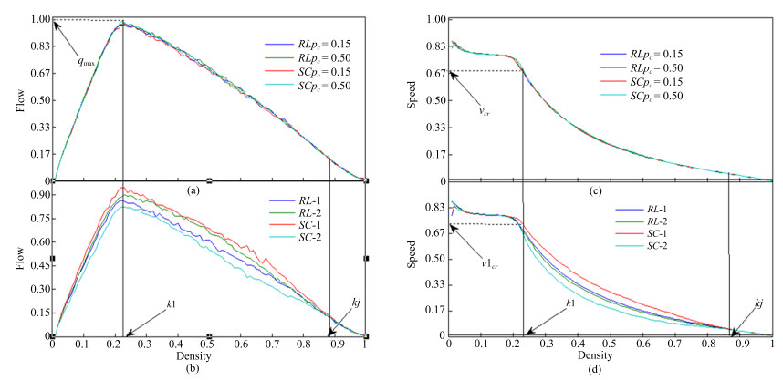
Fig. 1 is the fundamental and speed-density relation diagram of RL rule and SC rule. The traffic is in free flow and the interactions between vehicles on the road are very weak; thus, the average speed of vehicles on the road slightly decreases when the density increases from 0 to ${k_1}$. And the flow rate almost increases with the density in a fixed rate. At this time, the deviation of traffic flow (or vehicle speed) under different driving rules (or lane changing rate) is smaller than $2 %$ even under various operation rules and lane changing rates. The threshold flow rate is the maximum highway capacity and the vehicle speed $v_{cr}$ is the minimum speed in the free flow when the density value is ${k_1}$. But we denote the critical density required for separation of flow rate and average vehicle speed on the road when the individual rules come into effect by Figs. 1 (a) and 1 (c). The flow rate (vehicle speed) in Figs. 1 (b) and 1 (d) exist different kinds of curves with the increasing of density from ${k_1}$ to ${k_j}$. In RL rule, the vehicle accelerates to passing lane when it does not satisfy its current speed. And all when it does not satisfy its current speed. And all vehicles on passing lane will change to driving lane as soon as possible. So the flow rate (vehicle speed) on driving lane is naturally greater (weaker) than the flow rate on the other lane (Figs. 1 (b) and 1 (d)). In contrast, the vehicle speed (flow rate) on left lane is larger than the average velocity on right lane because of the different speed limitation under SC rule. At the same time, the traffic variables (including the flow rate and vehicle speed) under the SC rule is between the variables simulated from individual lane considering RL rule (Figs. 1 (b) and 1 (d)). The traffic jams naturally arise on account of the huge vehicles on the road. So the traffic variables under different operation rules are in agreement with the density increasing from ${k_{{j}}}$ (Fig. 1).

Figure  1.  The fundamental diagram: (a) and (c) are the flow-density plane and the speed-density plane; (b) and (d) are the flow-density plane on first and second lane and the speed-density plane on left and right lane (the passing rate is 0.15)

DownLoad: Full-Size Img PowerPoint

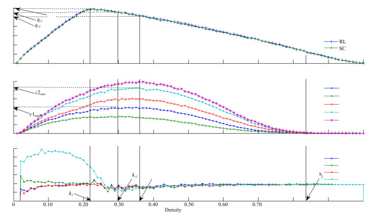
At the same lane changing rate and density, the lane changing times in the RL rule, due to the forced lane changing, is almost equal and greater than what we obtain under SC operation rule (Fig. 2 (b)). The maximum times of lane changing is at the point of congested flow (RL rule (${k_{c1}}$, ${q_{c1}}$), SC rule (${k_{c1}}$, ${q_{c1}}$). And there are ${k_{c1}} < {k_{c2}}$ and ${q_{c1}} < {q_{c2}}$ (Fig. 2 (a)). Furthermore, we analyze the total velocity deviation (Fig. 2 (c)). The results from various rules and lanes vary differently within the density range from 0 to ${k_1}$. If the density increase to ${k_{c2}}$, the speed population deviation is in an adjustment state and after that it maintains almost consistent. On the basis of the above analysis, spontaneously, we can not help wondering why the density of maximum times of lane changing do not agree with the greatest flow rate, why there exists adjusting regional of density and is there any relationship between them?

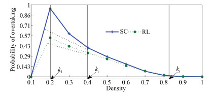
In this paper, we introduce the concept of lane changing probability introduced from the three phase traffic flow theory to explain the relationship mentioned above. First, we present the notion of lane changing probability [32].

Figure  2.  (a) The flow-density plane on left and right lane; (b) the times of lane changing; (c) the speed population deviation

DownLoad: Full-Size Img PowerPoint

where ${p_p}$ is the lane-changing probability, ${n_p}$ is the number of all vehicles that meet the conditions of lane-changing, and ${N_p}$ is the number of vehicles having lane changing motivation. Second, we try to clarify the differences between the lane changing rate and the lane changing probability. Apparently, the lane changing rate is ${p_c}$, which reflects the different type of drivers' types including radical type, neutral and so on. But ${p_p}$ represents the fundamental road condition whether a vehicle can make a lane changing.

The lane changing probability reaches the maximum ${k_1}$. So it is closely interrelated with the phase transition between the free flow and congested flow under the fundamental diagram approach in comparison with concept of lane changing rate. Besides, the value is always less than the other under RL rule (Fig. 3). This phenomenon shows that vehicles have better driving environment in SC rule. In addition, the absolute shape of lane changing probability has a large number of variety between ${k_1}$ and ${k_c}$ which means the driving conditions have deteriorated quickly. With the increasing of density from ${k_c}$ and ${k_j}$, the rate of lane changing probability remains the same. So we may explain the question and relationship as mentioned above.

Figure  3.  The probability of lane changing

DownLoad: Full-Size Img PowerPoint

Certainly, the research of lane changing rule will bring about road safety issues, and as a potential security risk, frequently lane changing often results in traffic safety hazard. In traffic engineering, researchers always aim to maximize the traffic flow, and at the same time ensure the security by reducing the potential risk of lane-changing times. Therefore, compared with RL rule, SC rule performs better.

Ⅳ. CONCLUSION

In this paper, two different traffic rules are respectively constructed to simulate the highway traffic flow. It is concluded that: the traffic flow and the average vehicle speed under the speed-limit rules and overtaking rules show few differences when they are having the same density. However, there are significant differences on different lanes under the congestion state; the lane-changing probability can preferably indicate the real conditions of the road, and the change of the lane-changing times will have some influence on the traffic flow; the speed limit rule can reduce lane-changing motivations and thus ensures the traffic safety on the highway effectively.

In further researches, firstly, the lane-changing probabilities and quantitative characteristics of mixed traffic flow are needed to be studied in detail to determine the numerical features of specific phase transition. Then, the metastable of the traffic flow under two different traffic rules needs to be further discussed. Finally, there are still many defects in this model which need to be improved, for example, the vehicle length, the number of lanes, and the rules of lane-changing, and honk effect, need to be further defined.