Figure
1.
Chaotic attractor of fractional Lorenz system with order α = 0.995.
 Volume 4
Issue 2
Volume 4
Issue 2
IEEE/CAA Journal of Automatica Sinica
| Citation: | Weiyuan Ma, Yujiang Wu and Changpin Li, "Pinning Synchronization Between Two General Fractional Complex Dynamical Networks With External Disturbances," IEEE/CAA J. Autom. Sinica, vol. 4, no. 2, pp. 332-339, Apr. 2017. doi: 10.1109/JAS.2016.7510202

|
FRACTIONAL calculus is as old as the conventional calculus. However, fractional calculus has become a hot topic in recent two decades due to its advantages in applications of physics and engineering. As a generalization of ordinary differential equation, fractional differential equation can capture non-local relations in space and time. Thus, the fractional-order models are believed to be more accurate than the integer-order models. Fractional models have been proven to be excellent instrument to describe the memory and hereditary properties of various materials and processes, such as dielectric polarization, electrode-electrolyte polarization, electromagnetic waves, viscoelastic systems, quantitative finance and waves [1]-[4].
It is demonstrated that fractional differential systems also behave chaotically or hyperchaotically, such as the fractional Lorenz system [5], the fractional Chua system [6], and the fractional Chen system [7]. Many complex networks usually consist of a large number of highly interconnected fractional dynamical units. Generally speaking, there are two main advantages of the fractional complex dynamical networks: one is infinite memory; the other is that the derivative order of a parameter enriches the system performance by increasing one degree of freedom. A fractional neural network is made up of thousands of neurons and their interactions. On the other hand, fractional differentiation provides neurons with a fundamental and general computation ability which can contribute to efficient information processing. Time delays are ubiquitous in neural networks due to finite switching speed of amplifiers. They usually occur in the signal transmission among neurons [8]-[10]. Therefore, it is more valuable and practical to investigate fractional complex networks with time delays.
Following these findings, synchronization of fractional chaotic systems becomes a challenging and interesting realm due to its potential applications in secure communication and control processing [11]-[16]. Many of complex networks normally have a large number of nodes, therefore it is usually expensive to control a complex network by designing the controllers for all nodes. To reduce the number of controllers, a pinning control method is proposed. Wang and Chen investigated a scale-free dynamical network by controlling a fraction of network nodes [17]. Sorrentino et al explored the pinning controllability of the complex networks [18]. Liang and Wang revealed the relationship between the coupling matrix and the synchronizability of complex networks via pinning control [19]. Yu et al studied synchronization via pinning control of general complex dynamical networks [20]. Nian and Wang investigated the optimal scheme of pinning synchronization of directed networks [21]. In addition, Liang and Wang proposed a method to quickly calculating pinning nodes on pinning synchronization in complex networks [22]. In [23]-[25], the authors investigated the pinning control of integer-order complex networks with time delays. However, pinning synchronization of integer-order complex networks was well-studied. Due to global dependent property of fractional complex networks, as far as we know, the literature on pinning synchronization of fractional complex networks is still sparse. In [26], based on the eigenvalue analysis and fractional stability theory, local stability properties of pinned fractional networks were derived. The pinning synchronization of new uncertain fractional unified chaotic systems were discussed in [27]. In [28], Chai et al proposed a global pinning synchronization for fractional complex dynamical networks. Xiang et al investigated the robust synchronization problem for a class of systems with external disturbances [29]. Wang et al provided a method to achieve projective synchronization of two fractional chaotic systems with external disturbances [30]. However, the effects of both time delay and external disturbance of the fractional complex network have seldom been considered.
Lyapunov direct method is important for synchronization analysis of complex networks with integer-order, but this method is difficult to be directly extended to fractional case [28], [31], [32]. Thus, to find out new ways to cope with these problems is still challenging. Motivated by the above discussions, pinning synchronization between the drive-response fractional complex networks with nonlinear coupling and time delays is studied. A novel modified Lyapunov method is used to analyze the global asymptotical synchronization criteria of fractional systems with time delays. These criteria rely on the coupling strength and the number of nodes pinned to the networks, there is no extra constraint on the two coupling matrices, such as symmetric or irreducible case.
The rest of this paper is arranged as follows. In Section Ⅱ, the general drive and response fractional complex dynamical network models are introduced and some necessary preliminaries are given. A Lyapunov-like criteria for delayed fractional system is obtained. In Section Ⅲ, based on the Lyapunov stability theorem, pinning controllers are designed to ensure the drive and response systems with external disturbances achieve synchronization. The illustrative numerical simulations are displayed in Section Ⅳ. Section Ⅴ concludes this paper.
Throughout this paper, let ‖ the Euclidean norm, I_n the identity matrix. If A is a vector or matrix, its transpose is denoted by A^{T} . Let \lambda_{\min}(A) and \lambda_{\max}(A) be the smallest and largest eigenvalue of symmetric matrix A, respectively.
In this section, we introduce some notations, definitions and preliminaries which will be used later on.
At present, there are several definitions of fractional differential operators [4], such as Grünwald-Letnikov definition, Riemann-Liouville definition, Caputo definition. Among them, the initial conditions for Caputo derivatives have the same form as those for integer-order ones. And Caputo derivative not only has a clearly interpretable physical meaning, but can also be properly measured to initializing in the simulation. So it may be the most appropriate choice for practical applications. Now we give the definition of Caputo fractional derivative _C D_{0, t}^{\alpha} f(t) , of order \alpha with respect to time t as follows
| \begin{eqnarray}\label{rb} _C D_{0, t}^{\alpha} f(t) =\frac{1}{\Gamma(m-\alpha)}\int_0^t(t-\tau)^{m-\alpha-1}f^{(m)}(\tau)d\tau \end{eqnarray} | (1) |
where m-1<\alpha<m\in\mathbb{Z}^+.
Consider a general fractional delayed dynamical system consisting of N nodes, which can be described as follows:
| \begin{align} _C D_{0, t}^{\alpha} x_i(t)=&\ Ax_i(t)+f(x_i(t))+c\sum_{j=1}^Nb_{ij}H x_j(t)\\ \label{dri} &\ +\bar{c}\sum_{j=1}^N\bar{b}_{ij}\bar{H}g(x_j(t-\tau))+\xi_i(t) \end{align} | (2) |
where i=1, 2, ..., N , 0<\alpha<1 is the fractional order, x_i(t)=(x_{i1}(t), ..., x_{in}(t))^{T} \in\mathbb{R}^n is the state variable of the i th node. A\in \mathbb{R}^{n\times n} is a given linear matrix, and f(x_i)= [f_1(x_{i}), f_2(x_{i}), ..., f_n(x_{i})]^{T}:\mathbb{R}^n\rightarrow \mathbb{R}^n is a smooth function describing the nonlinear dynamics of the node. c and \bar{c} are two parameters of the non-delay and delay coupling strengths, respectively. H\in\mathbb{R}^{n\times n} and \bar{H}\in\mathbb{R}^{n\times n} are inner coupling matrices. B=(b_{ij})_{N\times N} and \bar{B}=(b_{ij})_{N\times N} denote the coupling configuration matrices of the network. If there is a connection from node i to node j (i\neq j) , then b_{ij}>0 (or \bar{b}_{ij}>0 ); otherwise, b_{ij}=0 (or \bar{b}_{ij}=0 ). The diagonal elements of matrix B and \bar{B} are given by b_{ii}=-\sum_{j=1, j\neq i}^Nb_{ij} and \bar{b}_{ii}=-\sum_{j=1, j\neq i}^N\bar{b}_{ij} , respectively. g(x_i(t-\tau))= [g_1(x_i(t-\tau)), g_2(x_i(t-\tau)), ..., g_n(x_i(t-\tau))]^{T}:\mathbb{R}^n\rightarrow \mathbb{R}^n is the nonlinear coupling function. \xi_i(t)\in \mathbb{R}^{n} are external disturbance vectors.
If model (2) is referred as the drive system, the response complex network can be chosen as
| \begin{align} _C D_{0, t}^{\alpha} y_i(t)=&\ Ay_i(t)+f(y_i(t))+c\sum_{j=1}^Nb_{ij}H y_j(t)\\ \label{res} &\ +\bar{c}\sum_{j=1}^N\bar{b}_{ij}\bar{H}g(y_j(t-\tau))+\eta_i(t)+u_i(t) \end{align} | (3) |
where y_i(t)=(y_{i1}(t), y_{i2}(t), ..., y_{in}(t))^{T}\in \mathbb{R}^n is the response state vector of the i th node; \eta_i(t)\in \mathbb{R}^{n} are external disturbance vectors. u_i(t)\in \mathbb{R}^n (i=1, 2, ..., N) are the controllers to be designed; the other parameters have the same meanings as those in (2).
It is not necessary to assume that the inner coupling matrix H (or \bar{H} ) and coupling configuration matrix B (or \bar{B} ) are symmetric and irreducible. Meanwhile, the corresponding topological graph can be directed or undirected. Throughout the paper, we always assume that nonlinear functions f(x) and g(x) satisfy the uniform Lipschitz conditions,
| \left\| {f(x)-f(y)} \right\| \le L\left\| {x-y} \right\| | (4) |
| \left\| {g(x)-g(y)} \right\| \le \bar L\left\| {x-y} \right\|. | (5) |
We also assume the time-varying disturbances \xi_i(t) and \eta_i(t) are bounded and satisfy the following condition
| \begin{align} \|\xi_i(t)-\eta_i(t)\|\leq \tilde{L}_i\label{con3} \end{align} | (6) |
where \tilde{L}_i>0 .
According to systems (2) and (3), the error system is described by
| \begin{align} _C D_{0, t}^{\alpha} e_i(t)& = Ae_i(t)+f(y_i(t))-f(x_i(t))\\ & +c\sum_{j=1}^Nb_{ij}H e_j(t) +[\eta_i(t)-\xi_i(t)]+u_i(t)\\ \label{err} & +\bar{c}\sum_{j=1}^N\bar{b}_{ij}\bar{H}[g(y_j(t-\tau))-g(x_j(t-\tau))] \end{align} | (7) |
where e_i(t)=y_i(t)-x_i(t), i=1, 2, ..., N . Thus, our objective is to design a suitable controller u_i(t) such that error dynamical system (7) is asymptotically stable, i.e.,
| \lim_{t\rightarrow \infty}\|y_i(t; t_0, x_0)-x_i(t; t_0', x_0')\|=0, \quad i=1, 2, ..., N |
which implies the drive system (2) and the response system (3) are synchronized.
Now we present some lemmas for later use.
Lemma 1 [33]: Let x(0)=y(0) and _C D_{0, t}^{\alpha} x(t)\geq _CD_{0, t}^{\alpha} y(t) , where \alpha\in(0, 1) . Then x(t)\geq y(t) .
Lemma 2 [9], [10]: Consider the following linear fractional system with time delays:
| \begin{align}\label{eq} _C D_{0, t}^{\alpha} X(t)=AX(t)+X(t_\tau), \quad \alpha\in (0, 1) \end{align} | (8) |
where A=(a_{ij})_{n\times n} , X(t) =(x_1(t), x_2(t), ..., x_n(t))^{T} , X(t_\tau) =(\sum_{j=1}^nk_{1j}x_j(t-\tau_{1j}), \sum_{j=1}^nk_{2j}x_k(t- \tau_{2j}), ..., \sum_{j=1}^nk_{nj}x_j(t-\tau_{nj}))^{T}. Let M=(k_{ij}+a_{ij})_{n\times n} and B= (k_{ij}\exp(-s\tau_{ij}) +a_{ij})_{n\times n} . If all the eigenvalues of M satisfy |\arg(\lambda)|>\pi/2 and the characteristic equation \text{det}(\Delta(s))= |s^\alpha I_n-B|=0 has no purely imaginary roots for any \tau_{ij}> 0, i, j=1, 2, ..., n , then the zero solution of system (8) is Lyapunov asymptotically stable.
Lemma 3 [34]: Let x(t)=(x_1(t), ..., x_n(t))^{T}\in \mathbb{R}^{n} be a real continuous and differentiable vector function. Then
| _C D_{0, t}^{\alpha}[x^{T}(t)Px(t)]\leq 2x^{T}(t)P _C D_{0, t}^{\alpha} x(t) |
where 0<\alpha<1 , P is a symmetric and positive definite matrix.
Lemma 4 [35]: Let X and Y be arbitrary n -dimensional real vectors, K a positive definite matrix, and H\in \mathbb{R}^{n\times n} . Then, the following matrix inequality holds:
| \begin{equation*} 2X^{T}HY\leq X^{T}HK^{-1}X+Y^{T}KY. \end{equation*} |
Lemma 5 [36]: Assume that Q=(q_{ij})_{N\times N} is symmetric. Let M^*=\text{diag}\{m_1^*, m_2^*, ..., m_l^*, \underbrace{0, ..., 0}_{N-l}\} , 1\leq l\leq N , m_i^* > 0 ( i=1, 2, ..., l ), Q-M^*=\left( \begin{array}{cc} E-\widetilde{M}^* & S\\ S^{T} & Q_l\\ \end{array}\right) , \widetilde{M}^* = \text{diag}\{m_1^*, ..., m_l^*\} , m^*=\min_{1\leq i\leq l}\{m_i^*\} , Q_l is the minor matrix of Q by removing its first l (1\leq l\leq N) row-column pairs, E and S are matrices with appropriate dimensions. When m^*>\lambda_{\max}(E-SQ_l^{-1}S^{T}) , then Q-M^*<0 is equivalent to Q_l<0 .
Consider the Caputo fractional non-autonomous system with time delays
| \begin{align}\label{system} _C D_{0, t}^{\alpha}x(t)=f(t, x(t), x(t-\tau)) \end{align} | (9) |
with initial condition x(t)=x_0(t) , t\in [-\tau, 0] , where \alpha\in(0, 1) , f: [0, \infty)\times \Omega\rightarrow \mathbb{R}^n is piecewise continuous on t and locally Lipschitz with respect to x . \Omega \in \mathbb{R}^n is a domain that contains the origin x=0 . We always assume that (9) has an equilibrium x=0 .
It is well known, by using the Lyapunov direct method, we can get the asymptotic stability of the non-delays systems. Next, we extend the Lyapunov direct method to the time delays case, which leads to the Lyapunov asymptotic stability. Based on [9], [10], [33], we could obtain the following theorem.
Theorem 1: Let x=0 be an equilibrium point of system (9). If there exists a Lyapunov-like function V(t, x(t)):[-\tau, \infty] \times \Omega\rightarrow \mathbb{R} which is continuously differentiable and locally Lipschitz with respect to x such that
| {\alpha _1}{\left\| {x(t)} \right\|^a} \le V(t, x(t)) \le {\alpha _2}{\left\| {x(t)} \right\|^{ab}}\; | (10) |
| \begin{array}{l} CD_{0, t}^\alpha V(t, x(t)) \le-{\alpha _3}{\left\| {x(t)} \right\|^{ab}}\\ \qquad + {\alpha _4}{\left\| {x(t-\tau )} \right\|^a}\; \end{array} | (11) |
| \nu < \mu \sin \left( {\frac{{\alpha \pi }}{2}} \right) | (12) |
where a , b , \alpha_1 , \alpha_2 , \alpha_3 are positive constants, \mu={\alpha_3}/{\alpha_2} and \nu={\alpha_4}/{\alpha_1} . Then x=0 of system (9) is Lyapunov asymptotically stable.
Proof: It follows from (10) and (11) that
| \begin{align} &_C D_{0, t}^{\alpha} V(t, x(t))\\ &\qquad \leq-\frac{\alpha_3}{\alpha_2}V(t, x(t))+\frac{\alpha_4}{\alpha_1}V(t-\tau, x(t-\tau))\label{s3} \end{align} | (13) |
where t\geq 0 .
Consider the following system:
| \begin{align} &_C D_{0, t}^{\alpha} W(t, x(t))\\ &\qquad =-\mu W(t, x(t))+\nu W(t-\tau, x(t-\tau))\label{sj} \end{align} | (14) |
where W(t, x(t)) has the same initial conditions with V(t, x(t)) , \mu={\alpha_3}/{\alpha_2} and \nu={\alpha_4}/{\alpha_1} . Using Lemma 1, we have
| \begin{align}\label{6} 0\leq V(t, x(t))\leq W(t, x(t)). \end{align} | (15) |
By Lemma 2, the characteristic equation of (14) is \det (\Delta(s))=s^\alpha+\mu-\nu \exp(-s\tau)=0 . Suppose that s=\omega i = |\omega|(\cos({\pi}/{2})+i\sin(\pm {\pi}/{2})) . Substituting s into \det (\Delta(s)) gives
| \begin{align*} &|\omega|^\alpha\left(\cos\left(\frac{\alpha\pi}{2}\right)+i\sin\left(\pm \frac{\alpha\pi}{2}\right)\right)+\mu\\ &\qquad -\nu\left(\cos(\tau\omega)-i\sin(\tau\omega)\right)=0. \end{align*} |
Separating real and imaginary parts gives
| |\omega {|^\alpha }\cos \left( {\frac{{\alpha \pi }}{2}} \right) + \mu = \nu \cos \left( {\tau \omega } \right) | (16) |
| |\omega {|^\alpha }\sin \left( { \pm \frac{{\alpha \pi }}{2}} \right) =-\nu \sin \left( {\tau \omega } \right) | (17) |
According to (16) and (17), one has
| \begin{align}\label{9} |\omega|^{2\alpha}+2\mu\cos\left(\frac{\alpha\pi}{2}\right)|\omega|^\alpha+\mu^2-\nu^2=0. \end{align} | (18) |
Obviously, when \nu<\mu \sin({\alpha\pi}/{2}) , no real number \omega satisfies (18). Furthermore, the eigenvalue of M in equation is \nu-\mu . When \nu<\mu \sin({\alpha\pi}/{2}) , that is \nu<\mu , implying |\arg(\lambda(M))| > \pi/2 . So, W(t, x(t))\rightarrow 0 , as t\rightarrow +\infty .
From (15), V(t, x(t))\rightarrow 0 , as t\rightarrow +\infty , which means all the solutions of system (9) converge to x=0 .
In this section, some global asymptotically stable criteria are presented below.
To realize synchronization between (2) and (3), assume that first l (1\leq l\leq N) nodes are pinned, the pinning controllers are chosen as
| \begin{align}\label{cont} \begin{cases} u_i(t) = -p_ie_i(t)-q\dfrac{\text{sgn}(e_i(t))}{\sum\limits_{j=1}^n|e_{ij}(t)|},&1\leq i\leq l \\ u_i(t) = 0,& l+1\leq i\leq N \end{cases} \end{align} | (19) |
where p_i>0 are feedback gains, \text{sgn}(e_i(t))= (\text{sgn}(e_{i1}(t)), \text{sgn}(e_{i2}(t)), ..., \text{sgn}(e_{in}(t)))^{T} are signum vectors, and q= \frac{1}{2l}\sum_{i=1}^{N}\tilde{L}_i^2 .
Theorem 2: Suppose that the dynamical function f and nonlinear coupling function g satisfy Lipschitz conditions (4) and (5), respectively. If there exists a matrix P satisfying the following conditions
| \begin{array}{l} {\rm{1)}}\bar \mu =- {\lambda _{\max }}[\left( {a + L + \frac{1}{2} + \frac{{\bar c{\beta _2}\bar h(1 + \bar L)}}{2}} \right){I_N}\\ \;\;\;\;\;\;\;\;\;\; + ch\hat B-P] > 0 \end{array} | (20) |
| {\rm{2)}}\;\bar \nu < \bar \mu \sin \left( {\frac{{\alpha \pi }}{2}} \right) | (21) |
where a=\|A\|, h=\|H\|, \bar{h}=\|\bar{H}\|, \beta_1=\max\{\bar{b}_{ij}, j\neq i\}, \beta_2=\max\{|\bar{b}_{ii}|\} and \bar{\nu}=\frac{\bar{c}\bar{L}}{2}(N\beta_1\bar{L}+\bar{h}\beta_2) , then the fractional response network (3) asymptotically synchronizes to the drive network (2).
Proof: Construct the following Lyapunov-like function:
| \begin{align}\label{1} V(t, e(t))=\frac12\sum_{i=1}^Ne_i^{T}(t)e_i(t). \end{align} | (22) |
Using (7) and Lemma 3, the fractional derivative of V(t, e(t)) yields
| \begin{align}\label{2} _C D_{0, t}^{\alpha}& V(t, e(t))\leq\sum_{i=1}^Ne_i^{T}(t) _C D_{0, t}^{\alpha} e_i(t)\\ =&\ \sum_{i=1}^Ne_i^{T}(t)Ae_i(t)+\sum_{i=1}^Ne_i^{T}(t)[f(y_i(t))-f(x_i(t))]\\\ &+c\sum_{i=1}^N\sum_{j=1}^Nb_{ij}e_i^{T}(t)H e_j(t)+\sum_{i=1}^Ne_i^{T}(t)[\eta_i(t)-\xi_i(t)]\\ &+\bar{c}\sum_{i=1}^N\sum_{j=1}^N\bar{b}_{ij}e_i^{T}(t)\bar{H} [g(y_j(t-\tau))-g(x_j(t-\tau))]\\ &-\sum_{i=1}^lp_ie_i^{T}(t)e_i(t) -\sum_{i=1}^lq\frac{e^{T}_i(t)\text{sgn}(e_i(t))}{\sum\limits_{j=1}^n|e_{ij}(t)|}\\ \leq&\ (a+L)\sum_{i=1}^Ne_i^{T}(t)e_i(t)+c\sum_{i=1}^N\sum_{j=1}^Nb_{ij}e_i^{T}(t)H e_j(t)\\ &-\sum_{i=1}^lp_ie_i^{T}(t)e_i(t)-lq\\ &+\bar{c}\sum_{i=1}^N\sum_{j=1}^N\bar{b}_{ij}e_i^{T}(t) \bar{H}[g(y_j(t-\tau))-g(x_j(t-\tau))]\\ &+\sum_{i=1}^Ne_i^{T}(t)[\eta_i(t)-\xi_i(t)]. \end{align} | (23) |
From Lemma 4, we have (24), shown at the bottom of this page, and
| \begin{align}\label{3} &\sum_{i=1}^N\sum_{j=1}^N\bar{b}_{ij}e_i^{T}(t)\bar{H}\Big[g(y_j(t-\tau))-g(x_j(t-\tau))\Big]\\ \leq&\sum_{i=1}^N\sum_{j=1, j\neq i}^N\bar{b}_{ij}\Big[(g(y_j(t-\tau))-g(x_j(t-\tau)))^{T}(g(y_j(t-\tau))-g(x_j(t-\tau)))\\ &+ e_i^{T}(t)\bar{H}e_i(t)\Big]+2\bar{h}\bar{L}\sum_{i=1}^N|\bar{b}_{ii}|\cdot\|e_i(t)\|\cdot\|e_i(t-\tau)\|\\ \leq&\sum_{i=1}^N\sum_{j=1, j\neq i}^N\bar{b}_{ij}\Big[\bar{L}^2e_j^{T}(t-\tau)e_j(t-\tau)+\bar{h}e_i^{T}(t)e_i(t)\Big]\\ &+\bar{h}\bar{L}\sum_{i=1}^N|\bar{b}_{ii}|\Big[e_i^{T}(t)e_i(t)+e_i^{T}(t-\tau)e_i(t-\tau)\Big]\\ \leq&\ \beta_2\bar{h}(1+\bar{L})\sum_{i=1}^Ne_i^{T}(t)e_i(t) +\bar{L}(N\beta_1\bar{L}+\beta_2\bar{h})\sum_{i=1}^Ne_i^{T}(t-\tau)e_i(t-\tau) \end{align} | (24) |
| \begin{align}\label{4} \sum_{i=1}^N\sum_{j=1}^N&\ b_{ij}e_i^{T}(t)H e_j(t)\\ =& \sum_{i=1}^N\sum_{j=1, j\neq i}^Nb_{ij}e_i^{T}(t)H e_j(t)\\ &+\sum_{i=1}^Nb_{ii}e_i^{T}(t)\left(\frac{H+H^{T}}{2}\right)e_i(t)\\ \leq&\ h\sum_{i=1}^N\sum_{j=1, j\neq i}^Nb_{ij}\|e_i(t)\|\cdot\|e_j(t)\|\\ &+\rho_{\min}\sum_{i=1}^Nb_{ii}e_i^{T}(t)e_i(t) \end{align} | (25) |
where \rho_{\min} is the minimum eigenvalue of the matrix (H + H^{T})/{2} . Using Lemma 4 and (6), we get
| \begin{align}\label{j1} \sum_{i=1}^Ne_i^{T}&(t)[\eta_i(t)-\xi_i(t)]-lq\\ \leq &\ \frac12\sum_{i=1}^Ne_i^{T}(t)e_i(t)\\ &+\frac12\sum_{i=1}^N[\eta_i(t)-\xi_i(t)]^{T}[\eta_i(t)-\xi_i(t)]-lq\\ \leq &\ \frac12\sum_{i=1}^Ne_i^{T}(t)e_i(t)+\frac12\sum_{i=1}^N\tilde{L}_i^2-lq\\ =&\ \frac12\sum_{i=1}^Ne_i^{T}(t)e_i(t). \end{align} | (26) |
Substituting (24)−(26) into (23), and from Lemma 3, we obtain that
| \begin{align}\label{5} _C D_{0, t}^{\alpha}& V(t, e(t))\\ \leq&\ \|e(t)\|^{T}\bigg[\left(a+L+\frac12+\frac{\bar{c}\beta_2\bar{h}(1+\bar{L})}{2}\right)I_N\\ &+ch\hat{B}-P\bigg]\|e(t)\|\\ &+\frac{\bar{c}\bar{L}}{2}(N\beta_1\bar{L}+\bar{h}\beta_2)\|e(t-\tau)\|^{T}\cdot\|e(t-\tau)\|\\ \leq& -\bar{\mu} \sum_{i=1}^N e_i^{T}e_i(t)+\bar{\nu} \sum_{i=1}^N e_i(t-\tau)^{T}e_i(t-\tau) \end{align} | (27) |
where \|e(t)\|=(\|e_1(t)\|, \|e_2(t)\|, ..., \|e_N(t)\|)^{T} , P={\rm diag}(\underbrace{p_1, p_2, ..., p_l}_l, \underbrace{0, 0, ..., 0}_{N-l}) , \hat{B}=({\tilde{B}^{T}+\tilde{B}})/{2} and \tilde{B} is a modifying matrix of B via replacing the diagonal elements b_{ii} by (\rho_{\min}/h)b_{ii} .
According to Theorem 1, we have \|e_i(t)\|\rightarrow 0 , that is \|y_i(t)-x_i(t)\|\rightarrow 0 as t\rightarrow \infty , which means that the asymptotical synchronization between drive system (2) and response system (3) is realized.
Furthermore, from (27), let Q=(a+L+1/2+ {\bar{c}\beta_2\bar{h}}(1 + \bar{L})/{2})I_N+ch\hat{B} , and Q-P=\left( \begin{array}{cc} E-P^*&S\\ S^{T}&Q_l\\ \end{array} \right) , where 1 \leq l \leq N , P^*=\text{diag}\{p_1, p_2, ..., p_l\} , Q_l is the part matrix of Q by removing its first l row-column pairs, E and S are matrices with appropriate dimensions. Based on Lemma 5, and supposing that p_i (i=1, ..., l) are suitably large, Q-P<0 is equivalent to Q_l=[(a+L+1/2+ {\bar{c}\beta_2\bar{h}}(1+\bar{L})/{2})I_N+ch\hat{B}]_l < 0 . One has \lambda_{\max}[(a+L+1/2+{\bar{c}\beta_2\bar{h}}(1+\bar{L})/{2})I_N +ch\hat{B}]_l =(a+L+1/2+{\bar{c}\beta_2\bar{h}}(1+\bar{L})/{2}) +ch\lambda_{\max}(\hat{B}_l)<0 . So, the following corollary can be immediately obtained.
Corollary 1: Under assumptions (4) and (5), the fractional response network (3) asymptotically synchronizes to the drive one (2) under the controller (28), where p_i (i=1, ..., l) are sufficiently large, and the following conditions satisfied :
| \begin{align*} \mbox{ }~~\bar{\mu}=& -\bigg[\left(a+L+\frac12+\frac{\bar{c}\beta_2\bar{h}(1+\bar{L})}{2}\right)\\ &\ +ch\lambda_{\max}(\hat{B}_l)\bigg]>0\\ \mbox{ }~~\bar{\nu}<&\ \bar{\mu} \sin\left(\frac{\alpha\pi}{2}\right) \end{align*} |
in which \bar{\nu}=\frac{\bar{c}\bar{L}}{2}(N\beta_1\bar{L}+\bar{h}\beta_2) .
Corollary 2: If g(x_j(t-\tau))=x_j(t-\tau) and g(y_j(t-\tau))= y_j(t-\tau) , the synchronous conditions between (2) and (3) are reduced to:
| \begin{align*} \mbox{ }~~\bar{\mu}=& -\lambda_{\max} \bigg[\left(a+L+\frac{1}{2}+{\bar{c}\beta_2\bar{h}}\right)I_N\\ &\ + ch\hat{B}-P\bigg]>0\\[2mm] \mbox{ }~~\bar{\nu}<&\ \bar{\mu} \sin\left(\frac{\alpha\pi}{2}\right) \end{align*} |
where \nu=\frac{\bar{c}}{2}(N\beta_1+\bar{h}\beta_2) .
Corollary 3: Assume \xi_i(t)=\eta_i(t)=0 , the fractional complex networks (2) and (3) do not contain the disturbances. Under the assumptions (4) and (5), fractional systems (2) and (3) can be asymptotically synchronized under the controllers
| \begin{cases} u_i(t) = -p_ie_i(t), & 1\leq i\leq l \\ u_i(t) = 0, & l+1\leq i\leq N \end{cases} | (28) |
and the following control conditions:
| \begin{align*} \mbox{ }~~\bar{\mu}=& -\lambda_{\max}\bigg[\left(a+L+\frac{\bar{c}\beta_2\bar{h}(1+\bar{L})}{2}\right)I_N\\ &\ + ch\hat{B}-P\bigg]>0\\ \mbox{ }~~\bar{\nu}<&\ \bar{\mu} \sin\left(\frac{\alpha\pi}{2}\right) \end{align*} |
where \bar{\nu}=\frac{\bar{c}\bar{L}}{2}(N\beta_1\bar{L}+\bar{h}\beta_2) .
In this section, a numerical example is presented. Consider a complex network with 10 nodes, the fractional dynamical equation of each node is described by the following fractional chaotic Lorenz system
| \begin{align}\label{exa} \begin{cases} {_C D_{0, t}^{\alpha} x_{i1}} = a_L(x_{i2}-x_{i1})\\ {_C D_{0, t}^{\alpha} x_{i2}} = b_Lx_{i1}-x_{i1}x_{i3}-x_{i2} \\ {_C D_{0, t}^{\alpha} x_{i3}} = x_{i1}x_{i2}-c_Lx_{i3} \end{cases} \end{align} | (29) |
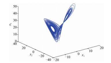
where i=1, 2, ..., 10 . The parameters are chosen as a_L=10, b_L=28, c_L=8/3 and \alpha=0.995 . From (2) and (3), we know that A=\left( \begin{array}{ccc} -a&a&0\\ b &-1&0\\ 0 &0 &-c \end{array} \right) , f(x_i(t))= \left( \begin{array}{c} 0\\ -x_{i1}x_{i3}\\ x_{i1}x_{i2} \end{array} \right) , and that system (29) is chaotic, see Fig. 1.
For convenience, let H=\bar{H}=I , the coupling configuration matrices B and \bar{B} are given as follows,
| \begin{eqnarray*} \left( \begin{array}{cccccccccc} -2 &1&0&1&0 &0&0 &0 &0 &0\\ 0 &-2&1&0&1 &0&0 &0 &0 &0\\ 1 &0&-3&0&0 &1&1 &0 &0 &0\\ 0 &0&1&-1&0 &0&0 &0 &0 &0\\ 0 &1&0&1&-3 &0&0 &0 &1 &0\\ 0 &0&1&0&1 &-2&0 &0 &0 &0\\ 0 &0&0&0&0 &1&-3 &1 &0 &1\\ 0 &1&0&1&0 &0&0 &-3 &1 &0\\ 1 &0&1&0&0 &0&1 &0 &-4 &1\\ 0 &0&1&1&0 &0&0 &0 &0 &-2 \end{array} \right). \end{eqnarray*} |
The nonlinear coupling function is chosen as
| \begin{align*} g(x_j(t-\tau))=&\ (x_{j1}(t-\tau)+\sin(x_{j1}(t-\tau)), \\ &\ x_{j2}(t-\tau)+\sin(x_{j2}(t-\tau)), \\ &\ x_{j3}(t-\tau)+\sin(x_{j3}(t-\tau)))^{T}. \end{align*} |
It is known that the Lorenz system is bounded. Actually, \|x_{i1}\|\leq 25, \|x_{i2}\|\leq 30, \|x_{i3}\|\leq 60, \|y_{i1}\|\leq 25, \|y_{i2}\|\leq 30, \|y_{i3}\|\leq 60, i=1, 2, ..., 10 , and
| \begin{align*} \|f(x_i)&-f(y_i)\|\\ \leq& ~\sqrt{(-x_{i1}x_{i3}+y_{i1}y_{i3})^2+(x_{i1}x_{i2}-y_{i1}y_{i2})^2}\\ \leq& ~75.83\|e_i\| \end{align*} |
that is L=75.83 . Obviously, \bar{L}=2 . According to the method proposed in [15], whose out-degrees are bigger than their in-degrees, it should be selected as pinned candidates. The out-degrees of nodes 2, 3 and 4 are bigger than their in-degrees, so we choose them as the pinned nodes. Rearrange the network nodes and the new order will be 4, 3, 2, 1, 6, 10, 5, 7, 8, 9.
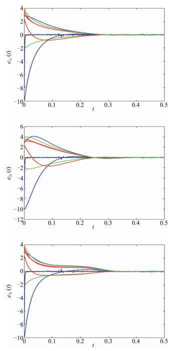
Under the no disturbance case, that is \xi_i(t)=\eta_i(t)=(0, 0, 0)^{T} , let p_i=910, i=1, 2, 3 , when \alpha=0.9, c=100, \bar{c} = 0.01 , one has \bar{\mu}\sin(\alpha\pi/2)=0.2808 and \bar{\nu}=0.2400 . From Corollary 3, it is clear that pinning conditions hold. The simulation results are shown in Fig. 2, which shows the time waveforms of errors e_{i1}, e_{i2}, e_{i3}, i=1, 2, ..., 10 . From the figures, fractional complex networks (2) and (3) are synchronized, which demonstrate the effectiveness of the proposed method.
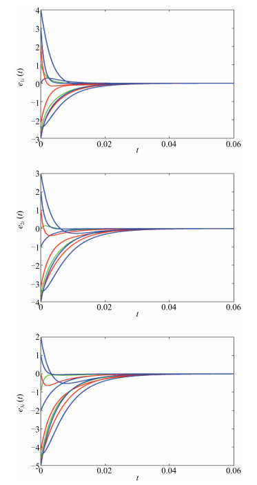
Now, we come to the disturbance case. Let p_i=930 , i= 1, 2, 3 , \xi_i(t)=(0, 0, 0)^{T} , \eta_i(t)=(0.3\sin t\cos t, 0.1\sin t , 0.5\cos t)^{T} , \alpha=0.9 , c=100 , \bar{c}=0.01 , one has q=0.5833 , \bar{\mu}\sin(\alpha\pi/2) =0.2489 and \bar{\nu}=0.2400 . From Theorem 2, it is clear that pinning conditions hold. Fig. 3 illustrates the synchronization phenomenon in noisy environment. It shows the error trajectories of drive and response networks, from which we can see that the synchronization between the driving and response networks is achieved successfully.

In this paper, we proposed a fractional pinning controller and presented a synchronization law for the delayed fractional complex networks with nonlinear couplings and disturbances. Some new synchronization criteria are proposed based on the Lyapunov-like stability theory. This method can be applied to many types of fractional complex networks. Furthermore, the coupling configuration matrices and the inner-coupling matrices are not assumed to be symmetric or irreducible. It means that this method is more general. The numerical results showed the effectiveness of the proposed controllers.
| [1] |
R. C. Koeller, "Polynomial operators, stieltjes convolution, and fractional calculus in hereditary mechanics, " Acta Mech. , vol. 58, no. 3-4, pp. 251-264, Apr. 1986. doi: 10.1007/s40243-015-0052-y
|
| [2] |
P. J. Torvik and R. L. Bagley, "On the appearance of the fractional derivative in the behavior of real materials, " J. Appl. Mech. , vol. 51, no. 2, pp. 294-298, Jun. 1984. https://utsa.influuent.utsystem.edu/en/publications/on-the-appearance-of-the-fractional-derivative-in-the-behavior-of
|
| [3] |
O. Heaviside, Electromagnetic Theory. New York, USA: Chelsea, 1971, pp. 1-130.
|
| [4] |
I. Podlubny, Fractional Differential Equations. New York, USA: Academic Press, 1998, pp. 201-307.
|
| [5] |
I. Grigorenko and E. Grigorenko, "Chaotic dynamics of the fractional Lorenz system, " Phys. Rev. Lett. , vol. 91, no. 3, pp. 034101, Jul. 2003. https://www.researchgate.net/publication/10624262_Chaotic_Dynamics_of_the_Fractional_Lorenz_System
|
| [6] |
T. T. Hartley, C. F. Lorenzo, and H. K. Qammer, "Chaos in a fractional order Chuaś system, " IEEE Trans. Circ. Syst. I Fund. Theory Appl. , vol. 42, no. 8, pp. 485-490, Aug. 1995. http://ieeexplore.ieee.org/document/404062/
|
| [7] |
C. G. Li and G. R. Chen, "Chaos in the fractional order Chen system and its control, " Chaos Solitons Fractals, vol. 22, no. 3, pp. 549-554, Nov. 2004. http://www.sciencedirect.com/science/article/pii/S0960077904001250
|
| [8] |
B. N. Lundstrom, M. H. Higgs, W. J. Spain, and A. L. Fairhall, "Fractional differentiation by neocortical pyramidal neurons, " Nat. Neurosci. , vol. 11, no. 11, pp. 1335-1342, Oct. 2008.
|
| [9] |
H. Wang, Y. G. Yu, G. G. Wen, S. Zhang, and J. Z. Yu, "Global stability analysis of fractional-order Hopfield neural networks with time delay, " Neurocomputing, vol. 154, pp. 15-23, Apr. 2015.
|
| [10] |
W. H. Deng, C. P. Li, and J. H. Lv, "Stability analysis of linear fractional differential system with multiple time delays, " Nonlinear Dyn. , vol. 48, no. 4, pp. 409-416, Jun. 2007. doi: 10.1007%2Fs11071-006-9094-0
|
| [11] |
C. P. Li, W. H. Deng, and D. Xu, "Chaos synchronization of the Chua system with a fractional order, " Phys. A: Stat. Mech. Appl. , vol. 360, no. 2, pp. 171-185, Feb. 2006. http://www.sciencedirect.com/science/article/pii/S0378437105007132
|
| [12] |
W. Y. Ma, C. P. Li, and Y. J. Wu, "Impulsive synchronization of fractional Takagi-Sugeno fuzzy complex networks, " Chaos: An Interdisciplinary J. of Nonlinear Sci. , vol. 26, no. 8, pp. 084311, 2016. doi: 10.1063/1.4959535
|
| [13] |
X. J. Wu and Y. Lu, "Generalized projective synchronization of the fractional-order Chen hyperchaotic system, " Nonlinear Dyn. , vol. 57, no. 1-2, pp. 25-35, Jul. 2009. http://www.wenkuxiazai.com/doc/086e81ef4afe04a1b071de23.html
|
| [14] |
L. P. Chen, Y. Chai, and R. C. Wu, "Linear matrix inequality criteria for robust synchronization of uncertain fractional-order chaotic systems, " Chaos Interdiscip. J. Nonlinear Sci. , vol. 21, no. 4, Article ID 043107, Oct. 2011. doi: 10.1063/1.3650237
|
| [15] |
Z. Odibat, "A note on phase synchronization in coupled chaotic fractional order systems, " Nonlinear Anal. Real World Appl. , vol. 13, no. 2, pp. 779-789, Apr. 2012. http://www.sciencedirect.com/science/article/pii/S1468121811002434
|
| [16] |
Y. C. Wang, H. G. Zhang, X. Y. Wang, and D. S. Yang, "Networked synchronization control of coupled dynamic networks with time-varying delay, " IEEE Trans. Syst. Man Cybern. B Cybern. , vol. 40, no. 6, pp. 1468-1479, Dec. 2010. http://ieeexplore.ieee.org/document/5422661/
|
| [17] |
X. F. Wang and G. R. Chen, "Pinning control of scale-free dynamical networks, " Phys. A: Stat. Mech. Appl. , vol. 310, no. 3-4, pp. 521-531, Jul. 2002. http://www.sciencedirect.com/science/article/pii/S0378437102007720
|
| [18] |
F. Sorrentino, M. di Bernardo, F. Garofalo, and G. R. Chen, "Controllability of complex networks via pinning, " Phys. Rev. E, vol. 75, no. 4, pp. 046103, Apr. 2007. http://www.nature.com/nature/journal/v473/n7346/full/nature10011.html
|
| [19] |
Y. Liang and X. Y. Wang, "Synchronizability on complex networks via pinning control, " Pramana, vol. 80, no. 4, pp. 593-606, Apr. 2013. http://cat.inist.fr/?aModele=afficheN&cpsidt=27102692
|
| [20] |
W. W. Yu, G. R. Chen, J. H. Lv, and J. Kurths, "Synchronization via pinning control on general complex networks, " SIAM J. Control Optim. , vol. 51, no. 2, pp. 1395-1416, Apr. 2013. doi: 10.1137/100781699
|
| [21] |
F. Z. Nian and X. Y. Wang, "Optimal pinning synchronization on directed complex network, " Chaos Interdiscip. J. Nonlinear Sci. , vol. 21, no. 4, pp. 043131, Dec. 2011. doi: 10.1063/1.3665699
|
| [22] |
Y. Liang and X. Y. Wang, "A method of quickly calculating the number of pinning nodes on pinning synchronization in complex networks, " Appl. Math. Comput. , vol. 246, pp. 743-751, Nov. 2014. https://www.deepdyve.com/lp/elsevier/a-method-of-quickly-calculating-the-number-of-pinning-nodes-on-pinning-UgjoEWItiW
|
| [23] |
Y. Liang, X. Y. Wang, and J. Eustace, "Adaptive synchronization in complex networks with non-delay and variable delay couplings via pinning control, " Neurocomputing, vol. 123, pp. 292-298, Jan. 2014. http://www.sciencedirect.com/science/article/pii/S0925231213007625
|
| [24] |
Y. H. Xu, C. R. Xie, and D. B. Tong, "Adaptive synchronization for dynamical networks of neutral type with time-delay, " Optik Int. J. Light Electr. Opt. , vol. 125, no. 1, pp. 380-385, Jan. 2014. http://www.sciencedirect.com/science/article/pii/S1468121806000861
|
| [25] |
R. R. Cheng, M. S. Peng, and W. B. Yu, "Pinning synchronization of delayed complex dynamical networks with nonlinear coupling, " Phys. A: Stat. Mech. Appl. , vol. 413, pp. 426-431, Nov. 2014. doi: 10.1063/1.2995852
|
| [26] |
Y. Tang, Z. D. Wang, and J. A. Fang, "Pinning control of fractional-order weighted complex networks, " Chaos Interdiscip. J. Nonlinear Sci. , vol. 19, no. 1, pp. 013112, Feb. 2009. doi: 10.1063/1.3068350
|
| [27] |
L. Pan, W. N. Zhou, J. A. Fang, and D. Q. Li, "Synchronization and anti-synchronization of new uncertain fractional-order modified unified chaotic systems via novel active pinning control, " Commun. Nonlinear Sci. Numer. Simul. , vol. 15, no. 12, pp. 3754-3762, Dec. 2010. http://www.sciencedirect.com/science/article/pii/S0960077907004316
|
| [28] |
Y. Chai, L. P. Chen, R. C. Wu, and J. Sun, "Adaptive pinning synchronization in fractional-order complex dynamical networks, " Phys. A: Stat. Mech. Appl. , vol. 391, no. 22, pp. 5746-5758, Nov. 2012. http://www.wenkuxiazai.com/doc/f62ead0bbed5b9f3f90f1c3a.html
|
| [29] |
W. Xiang and F. Q. Chen, "Robust synchronization of a class of chaotic systems with disturbance estimation, " Commun. Nonlinear Sci. Numer. Simul. , vol. 16, no. 8, pp. 2970-2977, Aug. 2011. doi: 10.1007%2F978-3-540-69307-9_3
|
| [30] |
D. F. Wang, J. Y. Zhang, and X. Y. Wang, "Robust modified projective synchronization of fractional-order chaotic systems with parameters perturbation and external disturbance, " Chin. Phys. B, vol. 22, no. 10, pp. 100504, Apr. 2013. http://cpb.iphy.ac.cn/EN/abstract/abstract55832.shtml
|
| [31] |
T. D. Ma and J. Zhang, "Hybrid synchronization of coupled fractional-order complex networks, " Neurocomputing, vol. 157, pp. 166-172, Jun. 2015. https://www.researchgate.net/publication/272375024_Hybrid_synchronization_of_coupled_fractional-order_complex_networks
|
| [32] |
L. X. Yang and J. Jiang, "Adaptive synchronization of drive-response fractional-order complex dynamical networks with uncertain parameters, " Commun. Nonlinear Sci. Numer. Simul. , vol. 19, no. 5, pp. 1496-1506, May2014. http://ieeexplore.ieee.org/document/7553164/
|
| [33] |
Y. Li, Y. Q. Chen, and I. Podlubny, "Mittag-Leffler stability of fractional order nonlinear dynamic systems, " Automatica, vol. 45, no. 8, pp. 1965-1969, Aug. 2009. http://dl.acm.org/citation.cfm?id=1746943
|
| [34] |
M. A. Duarte-Mermoud, N. Aguila-Camacho, J. A. Gallegos, and R. Castro-Linares, "Using general quadratic Lyapunov functions to prove Lyapunov uniform stability for fractional order systems, " Commun. Nonlinear Sci. Numer. Simul. , vol. 22, no. 1-3, pp. 650-659, May2015. http://www.sciencedirect.com/science/article/pii/S100757041400481X
|
| [35] |
J. S. Wu and L. C. Jiao, "Synchronization in complex delayed dynamical networks with nonsymmetric coupling, " Phys. A: Stat. Mech. Appl. , vol. 386, no. 1, pp. 513-530, Dec. 2007. http://www.sciencedirect.com/science/article/pii/S0378437107006024
|
| [36] |
Q. Song and J. D. Cao, "On pinning synchronization of directed and undirected complex dynamical networks, " IEEE Trans. Circ. Syst. I Regul. Pap. , vol. 57, no. 3, pp. 672-680, Mar. 2010. doi: 10.1007/s11071-010-9865-5
|

Figures(3)


Weiyuan Ma, Yujiang Wu and Changpin Li, "Pinning Synchronization Between Two General Fractional Complex Dynamical Networks With External Disturbances," IEEE/CAA J. Autom. Sinica, vol. 4, no. 2, pp. 332-339, Apr. 2017. doi: 10.1109/JAS.2016.7510202
 DownLoad:

 DownLoad: