

Figure
1.
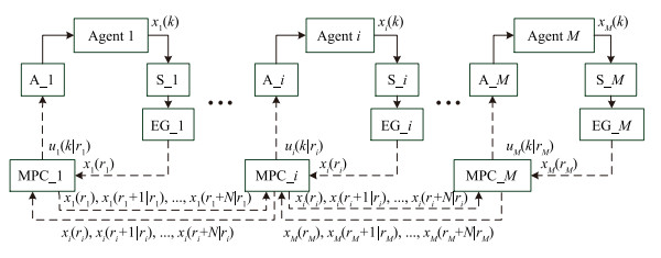
Structure of event-based MPC in wireless network.
 Volume 5
Issue 1
Volume 5
Issue 1
IEEE/CAA Journal of Automatica Sinica
| Citation: | Xiaoxiao Mi and Shaoyuan Li, "Event-triggered MPC Design for Distributed Systems With Network Communications," IEEE/CAA J. Autom. Sinica, vol. 5, no. 1, pp. 240-250, Jan. 2018. doi: 10.1109/JAS.2016.7510154

|
Although the wireless network can reduce the cabling cost and rapidly reconfigure the communication infrastructure in case of changing the system structure, the incorporation of this network into the distributed control poses new challenges to the control design.
On one hand, each local controller in the distributed systems decides on its current control action not only based on its own information, but also the shared information by others to improve the overall performance. These dynamical interaction among the controllers causes a tremendous amount of information transmitted through the network, especially when using the iterative algorithms [1], [2]. This increases the requirement for the network. On the other hand, the wireless nodes with limited battery power supply and limited bandwidth can't afford the mass transmission load and may lead to the network interruption, such that the system performance is degraded. In addition, it's shown that data transmission between nodes has an energy consumption much higher than the processing, and the energy consumption in the reception and idle states is of the same order of magnitude as in the transmission [3]. These considerations motivate the need of reducing the communication rate while promising the performance.
Lots of research have been done to deal with the problem aforementioned. From the angle of control design, event-triggered mechanism is introduced, which is different from the traditional time-triggered control. That is, in the event-triggered control, the wireless nodes perform their tasks if and only if an event occurs rather than the period manner. It avoids the unnecessary communication and realizes a good trade-off between the system performance and resources utilization.
Significant contributions have been made to the literature of event-triggered control, see [4]-[6] and the references therein. Specifically, a new method to design the triggering condition is presented based on the small-gain theorem for the nonlinear continuous systems in [5]. But the system states are continuously monitored in these event-triggered mechanisms. To further reduce the energy consumption of sampling, a self-triggered scheme is provided in [7]. Compared with the event-triggered control, the self-triggered control is proactive and computes the next sampling time or actuation instant ahead of time, so that the sensor nodes can keep in sleep mode before the predicted time. A periodic event-triggered control proposed in [8]-[9] can also avoid monitoring the triggering condition continuously. The event-triggered control strategy has developed rapidly and been applied to many fields recently [10]-[12]. [10] applied this strategy to the master-slave coupling systems with heterogeneous dimensions, thus the communication cost is reduced by only transmitting some of the states of the master system to the slave system. A co-design algorithm for determining the parameters of the triggering scheme and the consensus controller gain is also presented in [11]. Besides, the model predictive control (MPC) strategy is applied in [7] and a predictor is introduced in [8] to reduce communication by exchanging the predicted states with neighbors.
As well known, MPC is widely spread for control design of highly complex multi-variable processes with constraints. But as a receding horizon control method, the controller solves a finite horizon optimal problem every time, which motivates the event-triggered MPC study to reduce the unnecessary optimization, see [13]-[18]. It is shown that the practical implementation of wireless MPC based on event is validated, and is beneficial for experimental complex process in [15] with an operation on a divided wall column. Despite the vast literature on event-based control in the context of networked control systems, no results on event-based communication in distributed MPC are available at the moment [17], [18].
In this paper, we deal with the communication problem in the constrained distributed systems, consisting of linear time-invariant agents with a cooperated objective. The event-triggered MPC strategy is adopted, since it can not only reduce the transmission frequency, but also deal with system constraints and multi-objectives. The challenge is how to design a triggering condition to allow a substantial reduction of transmission without deteriorating the system performance.
The main contributions of this work are two-fold:
1) A triggering condition has been provided for the discrete-time linear systems based on the Lyapunov stability analysis. Here, to reduce the triggering times as much as possible, an event and transmission happen only when the Lyapunov function will exceed the value at the last updating time, and it may increase in few times, but an average decrease is guaranteed aiming at stabilizing the system.
2) Since the feasible region of the optimal control problem is very small with a short prediction time. But the accuracy of the predicted states decreases with the horizon length, and an overlarge prediction horizon affects the quickness of control scheme. Considering these cases, we optimize and minimize the terminal constrained set in the maximal control invariant ellipsoid set to expand the feasible region. And the stability is guaranteed as long as the initial state is feasible.
The organization of this paper is as follows. Section Ⅱ introduces the basic event-triggered MPC strategy. Then in Section Ⅲ, we propose an event-triggering condition, and design an event-triggered MPC strategy for the distributed system to reduce frequent communication. The feasibility and stability are also analyzed in Section Ⅲ. Finally, a simulation is provided to verify the theoretical results in Section Ⅳ. Section Ⅴ gives the conclusion and future directions of this research.
Notations: Throughout the paper, $\mathbb{R}^n$ denotes the $n$-dimensional Euclidean space. The notation $P\succ0$ means that matrix $P$ is a positive definite matrix. The symbol "$\ast$" denotes the symmetric term in a symmetric matrix. The superscripts "$T$" and "-1" represent the matrix transposition and inverse, respectively. The subscript "$i$" represents the $i$th agent. We use $\Vert\cdot\Vert$ to represent the Euclidean norm of a vector $x\in\mathbb{R}^n$ and also the induced norm of a matrix.
The distributed system considered consists of $M$ agents with a locally cooperating objective. The agents are modelled by the discrete-time linear system
| $$ \begin{equation} \mathit{\boldsymbol{x}}_i(k+1)=A_i\mathit{\boldsymbol{x}}_i(k)+B_i\mathit{\boldsymbol{u}}_i(k) \end{equation} $$ | (1) |
where $k\in\mathbb{Z}$ is the time step and $i=1, \ldots, M$, $\mathit{\boldsymbol{x}}_i(k)\in\mathbb{R}^{n_i}$ denotes the state of the $i$th subsystem at time $k$, and $u_i(k)\in\mathbb{R}^{m_i}$ the control input. $A_i$ and $B_i$ are constant matrices with appropriate dimensions. Besides, the control inputs are constrained in a compact set as $\mathit{\boldsymbol{u}}_i(k)\in\mathbb{U}_i$, and the states $\mathit{\boldsymbol{x}}_i(k)\in\mathbb{X}_i$. Both $\mathbb{U}_i$ and $\mathbb{X}_i$ contain the origin. Assume that the pair $(A_i, B_i)$ is controllable, and $(A_i, C_i)$ is observable.
In this paper, we focus on the communication network between sensors, controllers and the correlative agents. And each agent is controlled by an event-triggered MPC controller to reduce the communication rate over the wireless network, which forms a distributed MPC framework, see Fig. 1. The basic idea of this strategy is as follows.
Remark 1: In Fig. 1, "A$_i$" and "S$_i$" are short for actuator and sensor in the $i$th agent, respectively. $r_i$ denotes the last triggering time in the $i$th agent in Fig. 1. The sequence $\{{\mathit{\boldsymbol{x}}}_i(r_i), {\mathit{\boldsymbol{x}}}_i(r_i+1|r_i), \ldots, {\mathit{\boldsymbol{x}}}_i(r_i+N|r_i)\}$ is the information transmitted to its neighbors at the updating time $r_i$. The wireless communication channel among nodes considered in this work is represented by the dotted line.
At time step $k$, the wireless sensor nodes in the $i$th agent transmit the measurement $x_i(k)$ to its controller if and only if $||\mathit{\boldsymbol{x}}_i(k)-\tilde{\mathit{\boldsymbol{x}}}_i(k)||\geqslant\varepsilon_i$, where the design parameter $\varepsilon_i(>0)$ denotes the deviation threshold, $\tilde{\mathit{\boldsymbol{x}}}_i(k)$ shows the prediction of the current states. Then the $i$th agent solves a locally cooperated optimal problem (2) to determine its current control action, and transmits the corresponding predictive state trajectory to its neighbors.
| $$ \ \ \ \ \ \mathop {\rm min}\limits_{u_i(k)} J_i(\mathit{\boldsymbol{x}}_i(k), \mathit{\boldsymbol{u}}_i(k), \mathit{\boldsymbol{x}}_j(k))\nonumber\\ \ \ \ \ \ =\mathop{\rm min}\limits_{\mathit{\boldsymbol{u}}_i(k)} \sum\limits_{l=0}^{N-1}\Big[L_i(\tilde {\mathit{\boldsymbol{x}}}_i(k+l|k), \tilde {\mathit{\boldsymbol{u}}}_i(k+l|k))\nonumber\\ \ \ \ \ \ ~~~~\left.+ {\sum\limits_{j\in {N_i}}}H_{ij}(\tilde {\mathit{\boldsymbol{x}}}_i(k+l|k), \tilde {\mathit{\boldsymbol{x}}}_j(k+l|k))\right]\nonumber\\ \ \ \ \ \ ~~~~+V_{f_i}(\tilde {\mathit{\boldsymbol{x}}}_i(k+N|k))\\ {\text{s.t.}} ~~\tilde {\mathit{\boldsymbol{x}}}_i(k+l+1|k)=A_i\tilde {\mathit{\boldsymbol{x}}}_i(k+l|k)+B_i\tilde {\mathit{\boldsymbol{u}}}_i(k+l|k)\\ \ \ \ \ \ \ \ \ \ \ \ \ \ \ \ \ \ \ \ \ \ \ \ \ \ \ \ \ ~~~~l=0, \ldots, N-1\\ \ \ \ \ \ \ \ \ \ \ \ \ \ \ \ \ \ \ \ \ \ \ \ \ \ \ \ \ \tilde {\mathit{\boldsymbol{x}}}_i(k+l|k)\in\mathbb{X}_{i}\\ \ \ \ \ \ \ \ \ \ \ \ \ \ \ \ \ \ \ \ \ \ \ \ \ \ \ \ \ \tilde{\mathit{\boldsymbol{u}}}_i(k+l|k)\in\mathbb{U}_i \\ \ \ \ \ \ \ \ \ \ \ \ \ \ \ \ \ \ \ \ \ \ \ \ \ \ \ \ \ \tilde {\mathit{\boldsymbol{x}}}_i(k+N|k)\in X_f^i $$ | (2) |
where
| $$ \begin{gather} \begin{array}{lll} L_i(\tilde {\mathit{\boldsymbol{x}}}_i(k\!+\!l|k), \tilde {\mathit{\boldsymbol{u}}}_i(k\!+\!l|k))\!\triangleq\Vert\tilde{\mathit{\boldsymbol{x}}}_i(k\!+\!l|k)\Vert_{Q_i}^2\!\!+\!\!\Vert \tilde {\mathit{\boldsymbol{u}}}_i(k\!\!+\!\!l|k)\Vert_{R_i}^2\notag\\ %\end{eqnarray} H_{ij}(\tilde {\mathit{\boldsymbol{x}}}_i(k\!+\!l|k), \tilde {\mathit{\boldsymbol{x}}}_j(k\!+\!l|k))\!\triangleq\Vert\tilde {\mathit{\boldsymbol{x}}}_i(k\!+\!l|k)\!-\!\tilde {\mathit{\boldsymbol{x}}}_j(k\!+\!l|k)\Vert_{Q_{ij}}^2\notag\\ %\end{eqnarray} V_{f_i}(\tilde {\mathit{\boldsymbol{x}}}_i(k\!+\!N|k))\triangleq\Vert \tilde {\mathit{\boldsymbol{x}}}_i(k\!+\!N|k)\Vert_{P_i}^2 \notag \end{array} \end{gather} $$ |
$X_f^i$ is the target terminal set, and $\tilde {\mathit{\boldsymbol{x}}}_i(k|k)=\mathit{\boldsymbol{x}}_i(k)$. $Q_i, Q_{ij}$, $P_i$ and $R_i$ are the weighting matrices in the local cost function, coupling function, the terminal cost function and the input penalty, respectively. And assume that they all are symmetric positive definite matrices, denoted as $Q_i\succ0, Q_{ij}\succ0, P_i\succ0$ and $R_i\succ0$. The vector $\tilde {\mathit{\boldsymbol{x}}}_i(k+l|k)$ denotes the prediction states based on the measurement of the state at time $k$, which is a dependent variable and computed by solving the optimal problem. And $\mathcal{N}_{i}$ is a set of indexes of agents the $i$th agent communicates with, where $i\notin\mathcal {N}_i$.
It's worth noting that the threshold $\varepsilon_i$ is a critical tuning knob of the approach since it trades off the system performance and communication rate over the wireless channel. In this paper, our purpose is to design such a triggering condition to achieve a good trade-off. And we expect that the triggering condition can reduce the controller updating and communication resources largely, and also indicate the system performance dynamically.
In this section, the triggering condition will be provided based on the Lyapunov stability analysis. Then an improved scheme is put forward to expand the feasible region. And the whole control algorithm is introduced.
Firstly, some standard conditions for design parameters of the event-triggered MPC in distributed systems must be introduced, in order to assert that this strategy can result in a stabilizing controller.
Assumption 1: The stage function $L_i(\mathit{\boldsymbol{x}}_i, \mathit{\boldsymbol{u}}_i)$ is Lipschitz continuous in $\mathbb{X}_i\times\mathbb{U}_i$. That is, $\forall \mathit{\boldsymbol{x}}_{1_i}\in\mathbb{X}_i$ and $\mathit{\boldsymbol{x}}_{2_i}\in\mathbb{X}_i$, $\exists L_{Q_i}>0$,
| $$ \begin{eqnarray} s.t.~~\Vert L_i(\mathit{\boldsymbol{x}}_{1_i}, \mathit{\boldsymbol{u}}_{1_i})-L_i(\mathit{\boldsymbol{x}}_{2_i}, \mathit{\boldsymbol{u}}_{2_i})\Vert \leqslant L_{Q_i}\Vert \mathit{\boldsymbol{x}}_{1_i}-\mathit{\boldsymbol{x}}_{2_i}\Vert\notag. \end{eqnarray} $$ |
Assumption 2: The running cost $H_{ij}(\mathit{\boldsymbol{x}}_i, \mathit{\boldsymbol{x}}_j)$ is Lipschitz continuous in $\mathbb{X}_i\times\mathbb{X}_j$, with Lipschitz constants $L_{qx}^i$ and $L_{qx^a}^i$, respectively.
Assumption 3: There exists an invariant set, denoted as $\Phi_i\triangleq\{\mathit{\boldsymbol{x}}_i|\mathit{\boldsymbol{x}}_i^TP_i\mathit{\boldsymbol{x}}_i\leqslant \sigma^i, \sigma^i>0\}\subset\mathbb{X}_i$. And the terminal set $X_f^i\triangleq\{\mathit{\boldsymbol{x}}_i|\mathit{\boldsymbol{x}}_i^TP_i\mathit{\boldsymbol{x}}_i\leqslant \sigma_f^i, 0<\sigma_f^i\leqslant\sigma^i\}$, such that $0\in{X_f^i}\subset\Phi_i\subset\mathbb{X}_i$.
Assumption 4: If $\mathit{\boldsymbol{x}}_i(k)\in\Phi_i$, there exists a local stabilizing controller ${K_{f_i}}\mathit{\boldsymbol{x}}_i(k)\in {U_i}$, in the sense that $\tilde {\mathit{\boldsymbol{x}}}_i(k+1|k)=A_i\mathit{\boldsymbol{x}}_i(k)+B_iK_{f_i}\mathit{\boldsymbol{x}}_i(k)\in\Phi_i$. In addition, $\forall \mathit{\boldsymbol{x}}_i(k)\in X_f^i$, we have $\tilde {\mathit{\boldsymbol{x}}}_i(k+1|k)\in X_f^i$, and the associated terminal function has the following property
| $$ V_{f_i}(\tilde {\mathit{\boldsymbol{x}}}_i(k+1|k))-V_{f_i}(\mathit{\boldsymbol{x}}_i(k))\\ \ \ \ \ \ \leqslant-L_i(\mathit{\boldsymbol{x}}_i(k), \mathit{\boldsymbol{u}}_i(k))-\sum\limits_{j\in{N_i}}H_{ij}(\mathit{\boldsymbol{x}}_i(k), \mathit{\boldsymbol{x}}_j(k)). $$ |
Assumption 5: The terminal cost $V_{f_i}(\mathit{\boldsymbol{x}}_i)$ is Lipschitz continuous in $X_f^i$ with constant $L_{f_i}$.
Assumption 6: Idealize the wireless communication channel, neglect data loss and delays. Also, the latency and jitter issues are not considered in the wireless network.
For the system in (1), define the series $\{r_i\}(r_i\in\mathbb{N})$ as time instants when the optimization problem needs to be solved. The optimal control sequence and the optimal state trajectory at the triggering time $r_i$ are denoted by $\mathit{\boldsymbol{U}}_i^*(r_i)=[\mathit{\boldsymbol{u}}_i^*(r_i|r_i), \ldots, \mathit{\boldsymbol{u}}_i^*(r_i+N-1|r_i)]$, $\mathit{\boldsymbol{X}}_i^*(r_i)=[\mathit{\boldsymbol{x}}_i(r_i), \tilde {\mathit{\boldsymbol{x}}}_i^*(r_i+1|r_i), \ldots, \tilde {\mathit{\boldsymbol{x}}}_i^*(r_i+N|r_i)]$. At sampling time $r_i+m(m=1, $ … $, N-1)$, we construct a control trajectory $\bar {\mathit{\boldsymbol{U}}}_i(r_i+m)$ based on $\mathit{\boldsymbol{U}}_i^*(r_i)$, see (3). Concretely speaking, the corresponding inputs in $\mathit{\boldsymbol{U}}_i^*(r_i)$ are applied to the constructed predicted inputs during time $(r_i+m, r_i+N-1)$. After time $r_i+N$, the control action is computed by the feedback control law according to the predicted states. If no event is triggered at time $r_i+m$, take the current control action in (3); otherwise, update the control action by solving the optimization problem (2).
| $$ \bar {\mathit{\boldsymbol{u}}}_i(r_i+t|r_i+m)\\ =\left\{ \begin{array}{ll} %{ll}中的是小写的L,而不是数字1 \mathit{\boldsymbol{u}}_i^*(r_i+t|r_i), &t=1, \ldots, N-1 \\ {K_{f_i}}\tilde {\mathit{\boldsymbol{x}}}_i(r_i+t|r_i+m), &t=N, \ldots, N+m-1. \end{array} \right. $$ |
By recursive procedure, the feasibility of the control sequence $\bar U_i(r_i+m)$ can be easily proved as long as the initial state is in the feasible region. In addition, the designed control trajectory is independent of the states between time $r_i$ and $r_i+m-1$, so that this mechanism can be extended to a self-triggered formulation to avoid monitoring the states continuously.
With these preliminaries, a lemma is presented.
Lemma 1: Consider the system (1) with the optimal control problem (2). Suppose that Assumptions 1-6 hold, and the optimal problem of the $i$th agent is solved at time $r_i$, and the minimal index is $J_i^*(r_i)$. Define $\bar J_i(r_i+t)$ as the performance under the constructed feasible control actions (3). We have that, if there is no information received from its neighbors, the difference between $\bar J_i(r_i+t)$ and $J_i^*(r_i)$ is bounded by
| $$ \bar J_i(r_i+t)-J_i^*(r_i)\\ \ \ \ \ \ \ \leqslant\:L_{A1}(t)\Vert {\mathit{\boldsymbol{x}}}_i(r_i+t)-\tilde {\mathit{\boldsymbol{x}}}_i^*(r_i+t|r_i)\Vert-\sigma_{a_i}(t). $$ | (4) |
Otherwise,
| $$ \bar J_i(r_i+t)-J_i^*(r_i)\\ \ \ \ \ \ \leqslant\:L_{A2}(t)\Vert \mathit{\boldsymbol{x}}_i(r_i+t)-\tilde {\mathit{\boldsymbol{x}}}_i^*(r_i+t|r_i)\Vert-\sigma_{a_i}(t) \\ \ \ \ \ \ +\:\sum\limits_{l=t}^{N-1}\sum\limits_{j\in{\mathscr{N}_i}}L_{qx^a}^i\Vert\tilde {\mathit{\boldsymbol{x}}}_j(r_i+l|r_j^u)-\tilde {\mathit{\boldsymbol{x}}}_j(r_i+l|r_j)\Vert \notag $$ | (5) |
where
| $$ \begin{equation*} \begin{array}{l} L_{A1}(t)\triangleq L_{Q_i}\sum\limits_{l=t}^{N-1}\Vert A_i \Vert^{l-t}+L_{f_i}\Vert A_i\Vert^{N-t}\\~~~~~~~~~~~~+|\mathscr{N}_i|L_{qx}^i\sum\limits_{l=t}^{N-1} \Vert A_i \Vert^{l-t}\notag \end{array} \end{equation*} $$ |
| $$ \begin{equation*} \begin{array}{l}~\sigma_{a_i}(t) \triangleq \sum\limits_{l=0}^{t-1}\sum\limits_{j\in{\mathscr{N}_i}}H_{ij}(\tilde {\mathit{\boldsymbol{x}}}_i^*(r_i+l|r_i), \tilde {\mathit{\boldsymbol{x}}}_j(r_i+l|r_j)) \notag \\ ~~~~~~~~~~~+ \sum\limits_{l=0}^{t-1}L_i(\tilde {\mathit{\boldsymbol{x}}}_i^*(r_i+l|r_i), \mathit{\boldsymbol{u}}_i^*(r_i+l|r_i))\notag\\ ~L_{A2}(t) \triangleq L_{Q_i}\sum\limits_{l=t}^{N-1}\Vert A_i\Vert^{l-t}+L_{f_i}\Vert A_i \Vert^{N-t}\notag \end{array} \end{equation*} $$ |
$r_j\!=\!{\rm arg~min}_{r_j}{\{r_i-r_j>0\}}$ is the last triggering time of the $j$th agent at time $r_i$, and $r_j^u\!=\!{\rm arg~min}_{r_j}{\{r_i\!+\!t\!-\!r_j\!>\!0\}}$ is that of the $j$th agent at current time $r_i+t$. $|\mathscr{N}_i|$ denotes the number of its neighboring agents.
Proof: In this proof, we will prove that for any $t=1, \ldots, N-1$, the (4) or (5) always holds. First the inequality (4) is proved, and then the inequality (5) by the same procedure.
First, assume that there is no information received from its neighbors between time $r_i$ and $r_i+t$, thus the future states of its neighbors are all predicted based on the states at the same time. Then the performance difference between the cost functions at the current time and the last triggering time is
| $$ \bar J_i(r_i+t)-J_i^*(r_i)\\ \ \ \ \ {=}\:\sum\limits_{l=0}^{N-1}\Big[L_i(\tilde {\mathit{\boldsymbol{x}}}_i(r_i+t+l|r_i+t), \bar {\mathit{\boldsymbol{u}}}_i(r_i+t+l|r_i+t))\notag\\[-1mm] \ \ \ \ ~~{+}\:\sum\limits_{j\in {\mathscr{N}_i}}H_{ij}(\tilde {\mathit{\boldsymbol{x}}}_i(r_i+t+l|r_i+t), \tilde {\mathit{\boldsymbol{x}}}_j(r_i+t+l|r_j))\Big]\notag\\[-1mm] \ \ \ \ {+}\:V_{f_i}(\tilde {\mathit{\boldsymbol{x}}}_i(r_i+N+t|r_i+t))\notag\\[-1mm] \ \ \ \ {-}\:\sum\limits_{l=0}^{N-1}\Big[L_i(\tilde {\mathit{\boldsymbol{x}}}_i^*(r_i+l|r_i), \mathit{\boldsymbol{u}}_i^*(r_i+l|r_i))\notag\\[-1mm] \ \ \ \ ~~{+}\:\sum\limits_{j\in {\mathscr{N}_i}}H_{ij}(\tilde {\mathit{\boldsymbol{x}}}_i^*(r_i+l|r_i), \tilde {\mathit{\boldsymbol{x}}}_j(r_i+l|r_j))\Big]\notag\\[-1mm] \ \ \ \ {-}\:V_{f_i}(\tilde {\mathit{\boldsymbol{x}}}_i^*(r_i+N|r_i)) \\[-1mm] \ \ \ \ {=}\:\sum\limits_{l=t}^{N-1}\Big[L_i(\tilde {\mathit{\boldsymbol{x}}}_i(r_i+l|r_i+t), \bar {\mathit{\boldsymbol{u}}}_i(r_i+l|r_i+t))\notag\\[-1mm] \ \ \ \ ~~{-}\:L_i(\tilde {\mathit{\boldsymbol{x}}}_i^*(r_i+l|r_i), \mathit{\boldsymbol{u}}_i^*(r_i+l|r_i))\Big]\notag\\[-1mm] \ \ \ \ {+}\:\sum\limits_{l=N}^{N+t-1}\Big[L_i(\tilde {\mathit{\boldsymbol{x}}}_i(r_i+l|r_i+t), \tilde {\mathit{\boldsymbol{u}}}_i(r_i+l|r_i+t))\notag\\[-1mm] \ \ \ \ ~~{+}\:\sum\limits_{j\in{\mathscr{N}_i}}H_{ij}(\tilde {\mathit{\boldsymbol{x}}}_i(r_i+l|r_i+t), \tilde {\mathit{\boldsymbol{x}}}_j(r_i+l|r_j))\Big]\notag\\[-1mm] \ \ \ \ {+}\:V_{f_i}(\tilde {\mathit{\boldsymbol{x}}}_i(r_i+N+t|r_i+t))-V_{f_i}(\tilde {\mathit{\boldsymbol{x}}}_i^*(r_i+N|r_i)) \notag\\[-1mm] \ \ \ \ {+}\:\sum\limits_{l=t}^{N-1}\sum\limits_{j\in{\mathscr{N}_i}}H_{ij}(\tilde {\mathit{\boldsymbol{x}}}_i(r_i+l|r_i+t), \tilde {\mathit{\boldsymbol{x}}}_j(r_i+l|r_j))\notag\\[-1mm] \ \ \ \ {-}\:\sum\limits_{l=0}^{N-1}\sum\limits_{j\in{\mathscr{N}_i}}H_{ij}(\tilde {\mathit{\boldsymbol{x}}}_i^*(r_i+l|r_i), \tilde {\mathit{\boldsymbol{x}}}_j(r_i+l|r_j))\notag\\[-1mm] \ \ \ \ {-}\:\sum\limits_{l=0}^{t-1}L_i(\tilde {\mathit{\boldsymbol{x}}}_i^*(r_i+l|r_i), \tilde {\mathit{\boldsymbol{u}}}_i^*(r_i+l|r_i)).\notag $$ | (6) |
Based on (3), we have $\bar {\mathit{\boldsymbol{u}}}_i(r_i+l|r_i+t)=\mathit{\boldsymbol{u}}_i^*(r_i+l|r_i)$ for $l=t, \ldots, N-1$. By using the Assumption1, the difference for the stage cost can be bounded by
| $$ \begin{eqnarray} \sum\limits_{l=t}^{N-1}\Big[L_i(\tilde {\mathit{\boldsymbol{x}}}_i(r_i+l|r_i+t), \tilde {\mathit{\boldsymbol{u}}}_i(r_i+l|r_i+t))\notag\\ ~~{-}\:L_i(\tilde {\mathit{\boldsymbol{x}}}_i^*(r_i+l|r_i), \tilde {\mathit{\boldsymbol{u}}}_i^*(r_i+l|r_i))\Big]\notag\\ {\leqslant}\:L_{Q_{i}}\sum\limits_{l=t}^{N-1}\Vert\tilde {\mathit{\boldsymbol{x}}}_i(r_i+l|r_i+t)-\tilde {\mathit{\boldsymbol{x}}}_i^*(r_i+l|r_i)\Vert \notag\\ {=}\:L_{Q_{i}}\sum\limits_{l=t}^{N-1}\Vert A_i^{l-t}(\mathit{\boldsymbol{x}}_i(r_i+t)-\tilde {\mathit{\boldsymbol{x}}}_i^*(r_i+t|r_i))\Vert \notag\\ {\leqslant}\:L_{Q_{i}}\sum\limits_{l=t}^{N-1}\Vert A_i\Vert^{l-t}\Vert {\mathit{\boldsymbol{x}}}_i(r_i+t)-\tilde {\mathit{\boldsymbol{x}}}_i^*(r_i+t|r_i)\Vert. \end{eqnarray} $$ | (7) |
According to the Assumption 4, we get
| $$ L_i\Big[\tilde {\mathit{\boldsymbol{x}}}_i(r_i+N|r_i+t), \bar {\mathit{\boldsymbol{u}}}_i(r_i+N|r_i+t)\Big]\notag\\ {+}\:\sum\limits_{j\in{\mathscr{N}_i}}H_{ij}\Big[\tilde {\mathit{\boldsymbol{x}}}_i(r_i+N|r_i+t), \tilde {\mathit{\boldsymbol{x}}}_j(r_i+N|r_j)\Big]\notag\\ {+}\:V_{f_i}\Big[\tilde {\mathit{\boldsymbol{x}}}_i(r_i+1+N|r_i+t)\Big]\!\leqslant\! V_{f_i}\Big[\tilde {\mathit{\boldsymbol{x}}}_i(r_i\!+\!N|r_i+t)\Big]. $$ | (8) |
Similarly, a series of inequations can be found
| $$ \begin{eqnarray} &&~~L_i\Big[\tilde {\mathit{\boldsymbol{x}}}_i(r_i+N+h|r_i+t), \bar {\mathit{\boldsymbol{u}}}_i(r_i+N+h|r_i+t)\Big]\notag\\ &&~~{+}\:\sum\limits_{j\in{\mathscr{N}_i}}H_{ij}\Big[\tilde {\mathit{\boldsymbol{x}}}_i(r_i+N+h|r_i+t), \tilde {\mathit{\boldsymbol{x}}}_j(r_i+N+h|r_j)\Big]\notag\\ &&~~{+}\:V_{f_i}(\tilde {\mathit{\boldsymbol{x}}}_i(r_i+h+N+1|r_i+t)).\\ &&\leqslant\:V_{f_i}\Big[\tilde {\mathit{\boldsymbol{x}}}_i(r_i+N+h|r_i+t)\Big]\notag \end{eqnarray} $$ | (9) |
with $h=0, \ldots, t-1$.
Summing all the inequalities in (9), we have
| $$ \begin{eqnarray} &&~~\sum\limits_{l=N}^{N+t-1}\Big[L_i(\tilde {\mathit{\boldsymbol{x}}}_i(r_i+l|r_i+t), \tilde {\mathit{\boldsymbol{u}}}_i(r_i+l|r_i+t))\notag\\ &&~~~~{+}\:\sum\limits_{j\in{\mathscr{N}_i}}H_{ij}(\tilde {\mathit{\boldsymbol{x}}}_i(r_i+l|r_i+t), \tilde {\mathit{\boldsymbol{x}}}_j(r_i+l|r_j))\Big]\notag\\ &&~~{+}\:V_{f_i}(\tilde {\mathit{\boldsymbol{x}}}_i(r_i+N+t|r_i+t)) \notag\\ &&\leqslant\:V_{f_i}(\tilde {\mathit{\boldsymbol{x}}}_i(r_i+N|r_i+t)).\notag \end{eqnarray} $$ |
From the above deduction and the Assumption 5, the following inequality holds
| $$ \begin{eqnarray} &&~~\sum\limits_{l=N}^{N+t-1}\Big[L_i(\tilde {\mathit{\boldsymbol{x}}}_i(r_i+l|r_i+t), \tilde {\mathit{\boldsymbol{u}}}_i(r_i+l|r_i+t)) \notag\\ &&~~~~~~~~~~~{+}\:\sum\limits_{j\in{\mathscr{N}_i}}H_{ij}(\tilde {\mathit{\boldsymbol{x}}}_i(r_i+l|r_i+t), \tilde {\mathit{\boldsymbol{x}}}_j(r_i+l|r_j))\Big]\notag\\ &&~~{+}\:V_{f_i}(\tilde {\mathit{\boldsymbol{x}}}_i(r_i+N+t|r_i+t))-V_{f_i}(\tilde {\mathit{\boldsymbol{x}}}_i^*(r_i+N|r_i)) \notag\\ &&\leqslant\:V_{f_i}(\tilde {\mathit{\boldsymbol{x}}}_i(r_i+N|r_i+t))-V_{f_i}(\tilde {\mathit{\boldsymbol{x}}}_i^*(r_i+N|r_i)) \notag\\ &&\leqslant\:L_{f_i}\Vert\tilde {\mathit{\boldsymbol{x}}}_i(r_i+N|r_i+t)-\tilde {\mathit{\boldsymbol{x}}}_i^*(r_i+N|r_i)\Vert \notag\\ &&\leqslant\:L_{f_i}\Vert A_i\Vert^{N-t} \Vert \mathit{\boldsymbol{x}}_i(r_i+t)-\tilde {\mathit{\boldsymbol{x}}}_i^*(r_i+t|r_i)\Vert. \end{eqnarray} $$ | (10) |
Since there is no communication among the neighbors during time $(r_i, r_i+t)$, such that the predicted states of the neighbors are the same during time $(r_i+t, r_i+N-1)$. Then based on the Assumption 2, we have, for $l=t, \ldots, N-1$
| $$ \begin{eqnarray} &&~~H_{ij}(\tilde {\mathit{\boldsymbol{x}}}_i(r_i+l|r_i+t), \tilde {\mathit{\boldsymbol{x}}}_j(r_i+l|r_j))\notag\\ &&~~{-}\:H_{ij}( \tilde {\mathit{\boldsymbol{x}}}_i^*(r_i+l|r_i), \tilde {\mathit{\boldsymbol{x}}}_j(r_i+l|r_j)) \notag\\ &&\leqslant\:L_{qx}^i\Vert\tilde {\mathit{\boldsymbol{x}}}_i(r_i+l|r_i+t)-\tilde {\mathit{\boldsymbol{x}}}_i^*(r_i+l|r_i)\Vert. \notag \end{eqnarray} $$ |
Therefore,
| $$ \begin{eqnarray} &&~~\sum\limits_{l=t}^{N-1}\sum\limits_{j\in{\mathscr{N}_i}}H_{ij}(\tilde {\mathit{\boldsymbol{x}}}_i(r_i+l|r_i+t), \tilde {\mathit{\boldsymbol{x}}}_j(r_i+l|r_j))\notag\\ &&~~{-}\:\sum\limits_{l=0}^{N-1}\sum\limits_{j\in{\mathscr{N}_i}}H_{ij}( \tilde {\mathit{\boldsymbol{x}}}_i^*(r_i+l|r_i), \tilde {\mathit{\boldsymbol{x}}}_j(r_i+l|r_j)) \notag\\ &&\leqslant\:L_{qx}^i\sum\limits_{l=t}^{N-1}\sum\limits_{j\in{\mathscr{N}_i}}\Vert\tilde {\mathit{\boldsymbol{x}}}_i(r_i+l|r_i+t)-\tilde {\mathit{\boldsymbol{x}}}_i^*(r_i+l|r_i)\Vert \notag\\ &&~~{-}\:\sum\limits_{l=0}^{t-1}\sum\limits_{j\in{\mathscr{N}_i}}H_{ij}(\tilde {\mathit{\boldsymbol{x}}}_i^*(r_i+l|r_i), \tilde {\mathit{\boldsymbol{x}}}_j(r_i+l|r_j)) \notag\\ &&{\leqslant}\:|\mathscr{N}_i|\cdot L_{qx}^i\sum\limits_{l=t}^{N-1}\Vert A_i\Vert^{l-t}\Vert {\mathit{\boldsymbol{x}}}_i(r_i+t)-\tilde {\mathit{\boldsymbol{x}}}_i^*(r_i+t|r_i)\Vert \notag\\ &&~~{-}\:\sum\limits_{l=0}^{t-1}\sum\limits_{j\in{\mathscr{N}_i}}H_{ij}(\tilde {\mathit{\boldsymbol{x}}}_i^*(r_i+l|r_i), \tilde {\mathit{\boldsymbol{x}}}_j(r_i+l|r_j)). \end{eqnarray} $$ | (11) |
By summarizing the inequality (7), (10) and (11), the difference between the performance indexes is bounded, which completes the proof of inequality (4).
If the $j$th agent sends its current information to the $i$th subsystem at $r_j^u$, we get that, with the similar procedure
| $$ \begin{eqnarray} &&~~\sum\limits_{l=t}^{N-1}\sum\limits_{j\in{\mathscr{N}_i}}H_{ij}(\tilde {\mathit{\boldsymbol{x}}}_i(r_i+l|r_i+t), \tilde {\mathit{\boldsymbol{x}}}_j(r_i+l|r_j^u)) \notag\\ &&~~{-}\:\sum\limits_{l=0}^{N-1}\sum\limits_{j\in{\mathscr{N}_i}}H_{ij}(\tilde {\mathit{\boldsymbol{x}}}_i^*(r_i+l|r_i), \tilde {\mathit{\boldsymbol{x}}}_j(r_i+l|r_j)) \notag\\ &&\leqslant\:\sum\limits_{l=t}^{N-1}\sum\limits_{j\in{\mathscr{N}_i}}L^i_{qx^a}\Vert\tilde {\mathit{\boldsymbol{x}}}_j(r_i+l|r_j^u)-\tilde {\mathit{\boldsymbol{x}}}_j(r_i+l|r_j)\Vert\notag\\ &&~~{-}\:\sum\limits_{l=0}^{t-1}\sum\limits_{j\in{\mathscr{N}_i}}H_{ij}(\tilde {\mathit{\boldsymbol{x}}}_i^*(r_i+l|r_i), \tilde {\mathit{\boldsymbol{x}}}_j(r_i+l|r_j)). \end{eqnarray} $$ | (12) |
Summarizing the inequality (7), (10) and (12), the inequality (5) is proved.
Based on Lemma 1, the performance difference relates to the optimal state trajectory at the last triggering time and the current states. If we enforce the condition
| $$ \begin{eqnarray} \Vert {\mathit{\boldsymbol{x}}}_i(r_i+t)-\tilde {\mathit{\boldsymbol{x}}}_i^*(r_i+t|r_i)\Vert\leqslant\dfrac{\beta\sigma_{a_i}(t)}{L_{A1}(t)} \notag \end{eqnarray} $$ |
and
| $$ \begin{eqnarray} \sum\limits_{l=t}^{N-1}\sum\limits_{j\in{\mathscr{N}_i}}(L_{qx^a}^i\Vert\tilde {\mathit{\boldsymbol{x}}}_j(r_i+l|r_j^u)-\tilde {\mathit{\boldsymbol{x}}}_j(r_i+l|r_j)\Vert) \notag\\ +L_{A2}(t)\Vert {\mathit{\boldsymbol{x}}}_i(r_i+t)-\tilde {\mathit{\boldsymbol{x}}}_i^*(r_i+t|r_i)\Vert\leqslant\beta\sigma_{a_i}(t)\notag \end{eqnarray} $$ |
with $0<\beta<1$, we get $\bar J_i(r_i+t)< J_i^*(r_i)$. Thus, the event triggering condition of the $i$th agent is
| $$ \begin{eqnarray} \Vert {\mathit{\boldsymbol{x}}}_i(r_i+t)-\tilde {\mathit{\boldsymbol{x}}}_i^*(r_i+t|r_i)\Vert\geqslant\dfrac{\beta\sigma_{a_i}(t)}{L_{A1}(t)} \end{eqnarray} $$ | (13) |
or
| $$ \begin{eqnarray} \sum\limits_{l=t}^{N-1}\sum\limits_{j\in{\mathscr{N}_i}}(L_{qx^a}^i\Vert\tilde {\mathit{\boldsymbol{x}}}_j(r_i+l|r_j^u)-\tilde {\mathit{\boldsymbol{x}}}_j(r_i+l|r_j)\Vert) \notag\\ +L_{A2}(t)\Vert {\mathit{\boldsymbol{x}}}_i(r_i+t)-\tilde {\mathit{\boldsymbol{x}}}_i^*(r_i+t|r_i)\Vert\geqslant\beta\sigma_{a_i}(t). \end{eqnarray} $$ | (14) |
The triggering conditions (13) and (14) are just like a switch to determine whether the sensor sends the current information to the controller or not, and check if the neighboring agents exchange information with each other. At the initial time, the sensor transmits the system states to the controller and the neighboring agents exchange their states with each other to compute the control sequence and the predicted state trajectory. Then the triggering checking device stores the predicted states received from the controller. At the next time, the sensor measures the current states and check the conditions (13) and (14). Either (13) or (14) is satisfied, the states are sent to the controller and the problem (2) is solved, then the updated information is sent to its neighbors. Otherwise, this measurement is discarded, and the sensor waits for the next sampling. The control action input to the plant is still the predicted one at the last triggering time. Then move horizon to the next sampling time, and repeat the above process.
Remark 2: The triggering condition (13) or (14) is verified by the $i$th agent based on its current states, the predicted ones, and its neighboring predicted states. It can be seen as a distributed triggering condition. And the local controller may not solve the optimal problem while the triggering condition in its neighbors is satisfied.
Remark 3: It can be observed that the threshold is varying with time goes on, and may increase in a prediction horizon from the triggered time since $\sigma_{a_i}(t)$ is increasing but $L_{A1}(t)$ and the item about its neighboring states in the left side of inequality (14) decay with time goes on. However, it presents a decreasing trend due to the states gradually closing to the steady state. Here, the states threshold represents a tolerance to the maximal error of the predicted states while satisfying the stability condition. Therefore, triggering condition (13) or (14) is exactly the ways we expected, and can potentially save more computational and communication resources than the conditions in [17]. Because an event is triggered only when the performance index exceeds its value at the last updating time in this work, it leads to fewer triggering times than that of strategy in [17] where transmission happens if the cost function does not decrease successively at each sampling instants. However, it may take more time to reach the desired point because of relaxing the monotonicity.
Remark 4: In the implementation, we assume that the neighboring predicted states $\tilde {\mathit{\boldsymbol{x}}}_j(r_i+N+l|r_j)=\tilde {\mathit{\boldsymbol{x}}}_j(r_i+N|r_j), l=1, \ldots, N$.
Due to the accuracy of the predicted states decreases with the horizon length, an overlarge prediction horizon is unnecessary. Although the quickness is improved, MPC with a short prediction may cause infeasibility. It's also noted that the optimal solution may be infeasible with the aforementioned event-triggered MPC scheme because of constraints or disturbances. Considering these problems, we adopt the method with a series of asymptotically stable invariant ellipsoids in [19] to expand the feasible region. The difference is that we only optimize and minimize the terminal constrained set when the states are infeasible to the optimal problem (2), and the terminal penalty matrices $P_i$ is fixed.
Specifically, we first set a target terminal set $X_f^i$ and compute the maximal control invariant ellipsoid set $\Phi_i(X_f^i\subset\Phi_i)$, both $\Phi_i$ and $X_f^i$ satisfy the Assumptions 3 and 4. Solve the following minimization problem to steer the terminal set-valued state prediction $\tilde {\mathit{\boldsymbol{x}}}_i(r_i+N|r_i)$ into $X_f^i$. The state can always be controlled to the terminal set with this optimal problem if the initial state is feasible to $\Phi_i$, see [19]. Hence, the feasibility can be ensured all the time and feasible region is extended.
| $$ \begin{equation} \ \ \ \ \ \ \ \ \ \ \ \ \ \ \ \ \ \ \mathop {\rm min}\limits_{\alpha_i, U_i^*(k)} J_i(\mathit{\boldsymbol{x}}_i(k), \mathit{\boldsymbol{u}}_i(k), \mathit{\boldsymbol{x}}_j(k))\\ \ \ \ \ \ \ \ \ \ \ \ \ \ \ \ \ \ \ {\text{s.t.}}~~0\leqslant\alpha_i(k)\leqslant\alpha_i(k-1)\leqslant1 \\ \tilde {\mathit{\boldsymbol{x}}}_i(k+l|k)=A_i\tilde {\mathit{\boldsymbol{x}}}_i(k+l-1|k)+B_i\tilde {\mathit{\boldsymbol{u}}}_i(k+l-1|k)\\ \ \ \ \ \ \ \ \ \ \ \ \ \ \ \ \ \ \ \tilde{\mathit{\boldsymbol{x}}}_i(k+l|k)\in{X_i}, \qquad l=1, \ldots, N-1\\ \ \ \ \ \ \ \ \ \ \ \ \ \ \ \ \ \ \ \tilde {\mathit{\boldsymbol{u}}}_i(k+l|k)\in{U_i}, \qquad l=1, \ldots, N-1\\ \ \ \ \ \ \ \ \ \ \ \ \ \ \ \ \ \ \ \tilde {\mathit{\boldsymbol{x}}}_i(k+N|k)\in(1-\alpha_i)X_f^i+\alpha_i\Phi_i. \end{equation} $$ | (15) |
The triggering condition is designed similar as (13) and (14). And the whole control strategy for every subsystem can be described as Algorithm 1, taking the $i$th subsystem for example.
| Algorithm 1 Improved Event-triggered MPC |
| Step 1: At $r_i=0, k=0$, Initialization. Set $X_f^i$, compute $\Phi_i$, measure $x_i(0)$, and communicate with its neighbors, then solve the optimal problem (2). Finally, exchange $X_i^*(0)$. Let $k=k+1$. |
| Step 2: At time $k$, sample $x_i(k)$. If (13) or (14) is satisfied, turn to Step 4; else, turn to Step 3. |
| Step 3: If $k=r_i+N$, turn to Step 4. Otherwise, apply the corresponding control action $u_i^*(k|r_i)$ to the plant, turn to Step 5. |
| Step 4: Solve problem (2) or (15), apply the current control action $u_i^*(k)$ to the local subsystem, send $X_i^*(k)$ and turn to Step 6. |
| Step 5: Wait for the next sampling, let $k=k+1$ and turn to Step 2. |
| Step 6: Let $r_i=k$, move horizon to the next sampling, that is $k=k+1$, and turn to Step 2. |
 DownLoad:
CSV
DownLoad:
CSV
Remark 5: If controllers in the the subsystems are triggered synchronously, we adopt an iterative algorithm to realize agent negotiation.
Remark 6: The optimal problem (15) is solved only if there is no feasible solution to the problem (2) in this paper. If the problem (2) is replaced by the problem (15) with the same parameters in the implementation, the triggering times are less than that of using the problem (2), but the cost values are relatively larger.
In this section, the feasibility and stability analysis of the proposed control strategy is going to be given. To ensure that there exists a solution satisfying all the constraints when there is an event, the feasibility is provided. Then, it's proven the closed-loop system is Lyapunov Stable.
Theorem 1: Consider the system described by (1), and suppose that Assumptions 1-6 hold, the control actions are generated by Algorithm 1 with triggering condition (13) and (14). We have that the system state converges to the terminal set in finite time as long as the initial state is feasible.
Proof: In this paper, a state predicted trajectory is evaluated after measuring the current state. And if the predicted states at the prediction horizon $\tilde {\mathit{\boldsymbol{x}}}_i(k+N|k)$ exceeds the terminal set $X_f^i$, we solve the optimal problem (15). Then we can construct a feasible control sequence based on the optimal solution at $k$, see (3), so that the optimal terminal set becomes closer to the target one recursively. Therefore, the control action is always feasible. At the triggering time $r_i$, the cost function is $J_i^*(r_i)$. At time instant $r_i+l$, based on the triggering condition (13) and (14), the cost value corresponding to the feasible input satisfies $\bar J_i(r_i+l)\leqslant J_i^*(r_i)$. Then we have $J_i^*(r_i+l)\leqslant J_i^*(r_i)$, and the system converges to the terminal set in finite time.
There are lots of parameters in this algorithm that significantly affect the system performance. The guidance to their selection is provided in this part.
1) Parameters in the Optimal Problem: As well known, the prediction horizon $N$ can trade off the system stability and rapidity, and also act as the maximal triggering interval in this paper. Since the mentioned algorithm can improve the system performance than traditional MPC with a short prediction horizon, but the computation burden and complexity are not reduced if $N$ is larger. Hence, the prediction horizon $N$ selected can't be overlarge. The control horizon here is equal to the prediction horizon. Besides, the weighting matrices $Q_i, Q_{ij}, R_i$ are symmetric positive definite matrices. The greater the elements in these matrices, the smaller the corresponding optimal variables obtained. Thus these matrices can be chosen based on the practical demands. The matrix $P_i$ and the feedback control gain $K_{f_i}$ chosen should ensure that the Assumptions 3 and 4 hold, and can be obtained by means of linear matrix inequalities concept [20].
2) Parameters in the Assumptions 1-5: Firstly, $\sigma_i$ shows the region of the initial feasible set, and $ \sigma_f^i$ in the target terminal set represents the final convergence of the system. The smaller $\sigma_f^i$, the closer system state tends to the desired point. Detailedly, after choosing the target terminal set, we can obtain $\sigma_i$ by using the $i$-step controllable set [21]. Then, $L_{Q_i}, L_{qx}^i, L_{qx^a}^i, L_{f_i}, K_{f_i}$ are computed by trial-anderror method. The design paramete $\beta_i$ in the triggering condition is selected in $(0, 1)$. It has a significant influence on the trade-off between the system stability and communication rates. The condition (13) and (14) with a smaller $\beta_i$ lead to more frequent communication, but the system performance obtained is better.
This section illustrates the performance of the proposed Algorithm 1 in simulation. Consider a discrete LTI system consisting of 3 agents with a cooperative objection, where the system matrices are as follows:
| $$ \begin{eqnarray} A_1=\left[ \begin{array}{cc} 1&0.2\notag\\ -0.5&-0.4 \end{array} \right], A_2=\left[ \begin{array}{cc} 1&0.2\notag\\ -1.2&-0.2 \end{array} \right]\notag\\ A_3=A_2, B_3=B_2=B_1=[0, 0.2]^T.~~~~~~~\!~~~~~~~\notag \end{eqnarray} $$ |
The state and control constraints are $\|x_i\|_2\leqslant5, \|u_i\|_2\leqslant1$. Based on the principles in Section Ⅲ, the tuning parameters for each agent are set with $N=5, Q_1=Q_2=Q_3=I_2, R_1=R_2=R_3=I_1, Q_{12}=Q_{13}=0.5I_2, Q_{21}=Q_{31}=I_2$. To satisfy the Assumptions 3 and 4, we set $\sigma_f^1=1, \sigma_f^2=1, \sigma_f^3=1$, then $\sigma^1=36, \sigma^2=33, \sigma^3=33$, and the matrices $P_i, K_i(i=1, 2, 3)$ are obtained.
| $$ \begin{gather} P_1=\left[ \begin{array}{cc} 12.1548&2.0205\notag\\ 2.0205&1.8282 \end{array} \right], P_2=P_3=\left[ \begin{array}{cc} 9.7642&2.0592\notag\\ 2.0592&1.769 \end{array} \right]\notag\\ K_1=[-0.2861, 0.0185], K_2=K_3=[0.0643, -0.0011].~~~~~~\notag \end{gather} $$ |
The other parameters required are numerically found, such as, $L_{Q_1}=67, L_{Q_2}=47, L_{Q_3}=47, L_{f_1}=13, L_{f_2}=16, L_{f_3}=9,$$L_{qx}^1=19, L_{qx}^2=32, L_{qx}^3=3, L_{qx^a}^1=24,$$L_{qx^a}^2=31, L_{qx^a}^3=31, \beta_1=0.87, \beta_2=0.9, \beta_3=0.9$.
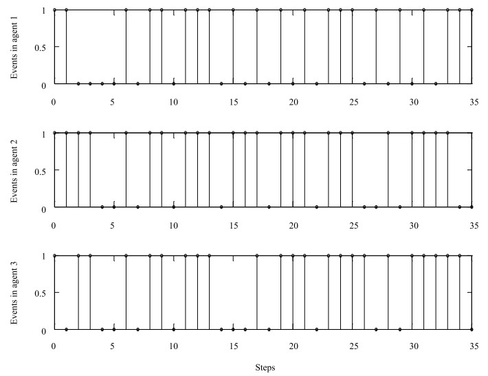
First, we execute the proposed Algorithm 1 at the feasible initial states $\mathit{\boldsymbol{x}}_1(0)=[0.5, 0.5]^T, \mathit{\boldsymbol{x}}_2(0)=[-1, -2]^T, \mathit{\boldsymbol{x}}_3(0)=[0, 3]^T$ with a small disturbances $w_i, \Vert w_i\Vert\leqslant0.05, i=1, 2, 3$. Then the states trajectories, cost function values and the triggering instants, shown in Figs. 2-6, are compared with that of the traditional distributed MPC (DMPC) with an iterative scheme [1] and the event-based MPC in [17] for a linear distributed system.

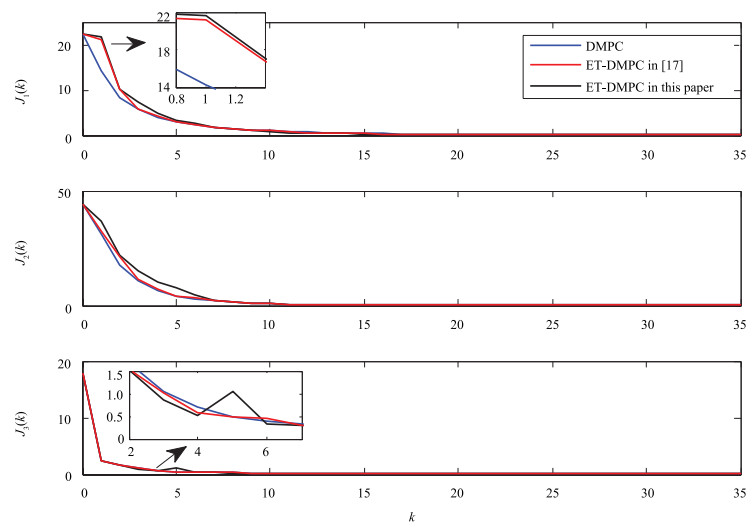
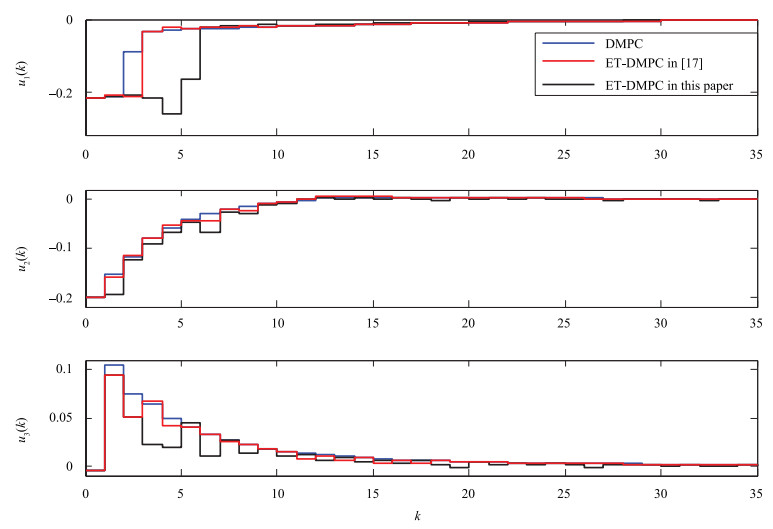
As is shown in Fig. 2, the optimal state trajectory with Algorithm 1 is well coincided with the trajectory under traditional DMPC, but there is a smaller deviation between the trajectory with strategy in [17] and the traditional DMPC. It's observed from Fig. 3 that the performance index decays slowly, and even increases at the Steps 1 and 5 with Algorithm 1, while it decreases successively with the event-triggered MPC strategy in [17] and traditional DMPC.
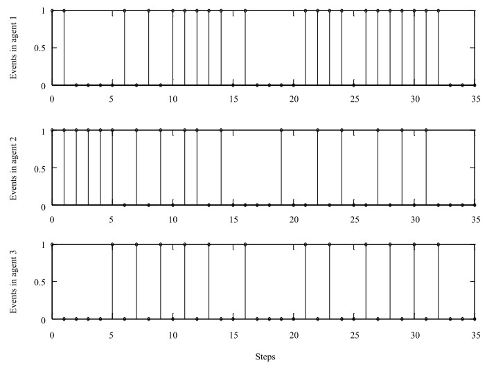
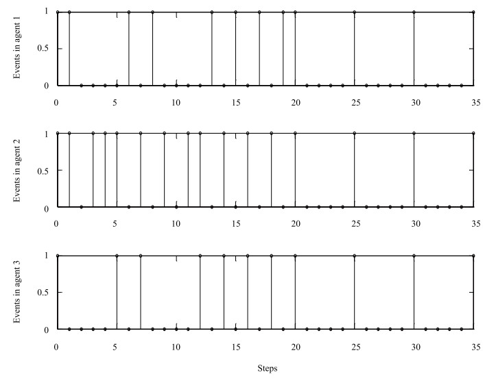
In addition, in Figs. 5, 6, and 8, "1" denotes that an event occurs at this step, and the corresponding agents communicate with each other; otherwise, "0" shows that the triggering condition is not satisfied, and there is no communication between these agents. It's easily observed that the less the number of "1" in Figs. 5, 6 and 8, the more communication resources saving. Contrasting Fig. 5 with Fig. 6, we can obtain that with the proposed Algorithm 1, the event between sensor and controller occurs 21 times in 35 simulation steps in the first agent, the number of events in the $2$th agent and $3$th agent are 17 and 13, respectively. We can get that with the event-triggered MPC in [17], the controllers in the first agent, the $2$th agent and $3$th agent are triggered 21, 24, 23 times, respectively. Obviously, the triggering event happens less frequently than that of the event-triggered MPC in [17]. Besides, in this paper, the controller in the first agent exchanges information with its neighbors 29 times, communication with neighbors for the 2th agent and 3th agent are 29 times and 23 times, respectively, while a tremendous amount of information is transmitted among these 3 agents caused by 102 times iterative calculation in the traditional DMPC. Hence, it saves more energy on computation and transmission over neighbors wireless network with Algorithm 1.
Therefore, the proposed method realizes a good trade-off between communication rate and the system performance.
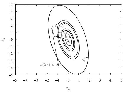
Then, to illustrate the feasibility expansion with adaptive terminal set, we take $\mathit{\boldsymbol{x}}_1(0)=[-1, -3]^T, \mathit{\boldsymbol{x}}_2(0)=[1, -2]^T, \mathit{\boldsymbol{x}}_3(0)=[0, -3]^T$ for example, which is called infeasible states due to terminal constraints violation in the $1$th agent. As shown in Fig. 7, we get a series of minimal and optimal sets by solving the problem (15) at the time Steps 1, 2, 6 and 8, which are gradually narrowing to the set terminal set $X_f$. Finally, the agent states are steered to the desired position. Besides, the triggering instants are shown in Fig. 8. It can be seen that the triggering condition (13) or (14) is always unsatisfied with the system gradually closing to the steady states, and it tends to control periodically whose period is equal to the prediction horizon.
In conclusion, the simulation results verify the effectiveness of the proposed Algorithm 1.
Remark 6: In Fig. 7, $"C_1$" represents the control invariant set $\Phi_1$ in the first agent with the largest ellipse, $"X_f$" denotes the target terminal set with the minimal one, the others are the optimal terminal sets solved by problem (15) at time $k$=1, 2, 6 and 8, when the optimal problem (2) is infeasible. After time 13, the terminal set keeps $X_f$.
This paper presented an event-triggered MPC design algorithm for the distributed systems consisting of linear discrete time-invariant agents. We first described the basic event-triggered MPC control strategy, then proposed a triggering condition based on the Lyapunov stability analysis intended to reduce the communication over wireless network largely. The condition proposed caused that the Lyapunov function non-monotonically declined, but was enforced not to exceed the value at the last triggered time. It's different from the other method where the Lyapunov function decreased successively. Then the feasible region was expanded by adjusting the terminal set dynamically and the control algorithm based on these was given. Simulation results had validated the effectiveness of the proposed strategy.
The self-triggered scheme may be developed in the future study to reduce the idle states, and keep the nodes in sleep mode until transmission is required. And we will present different terminal criterion in the iterative algorithm using the event-triggered mechanism.
| [1] |
R. Scattolini, "Architectures for distributed and hierarchical model predictive control-a review, " J. Process Control, vol. 19, no. 5, pp. 723-731, May 2009. http://www.sciencedirect.com/science/article/pii/S0959152409000353
|
| [2] |
J. M. Maestre, D. M. De La Pe?na, E. F. Camacho, and T. Alamo, "Distributed model predictive control based on agent negotiation, " J. Process Control, vol. 21, no. 5, pp. 685-697, Jun. 2011. http://www.sciencedirect.com/science/article/pii/S0959152410002404
|
| [3] |
G. Anastasi, M. Conti, M. Di Francesco, and A. Passarella, "Energy conservation in wireless sensor networks:a survey, " Ad Hoc Networks, vol. 7, no. 3, pp. 537-568, May 2009.
|
| [4] |
W. P. M. H. Heemels, K. H. Johansson, and P. Tabuada, "An introduction to event-triggered and self-triggered control, " in Proc. 2012 IEEE 51st Annu. Conf. Decision and Control, Maui, USA, 2012, pp. 3270-3285. http://ieeexplore.ieee.org/xpls/icp.jsp?arnumber=6425820
|
| [5] |
T. F. Liu and Z. P. Jiang, "A small-gain approach to robust eventtriggered control of nonlinear systems, " IEEE Trans. Automat. Control, vol. 60, no. 8, pp. 2072-2085, Aug. 2015. http://ieeexplore.ieee.org/document/7027161/
|
| [6] |
T. F. Liu and Z. P. Jiang, "Event-based control of nonlinear systems with partial state and output feedback, " Automatica, vol. 53, pp. 10-22, Mar. 2015. http://www.sciencedirect.com/science/article/pii/S0005109814006062
|
| [7] |
T. M. P. Gommans and W. P. M. H. Heemels, "Resource-aware MPC for constrained nonlinear systems:a self-triggered control approach, " Syst. Control Lett., vol. 79, pp. 59-67, May 2015. http://www.sciencedirect.com/science/article/pii/S0167691115000481
|
| [8] |
W. P. M. H. Heemels and M. C. F. Donkers, "Model-based periodic event-triggered control for linear systems, " Automatica, vol. 49, no. 3, pp. 698-711, Mar. 2013. http://www.sciencedirect.com/science/article/pii/S0005109812005614
|
| [9] |
W. P. M. H. Heemels, M. C. F. Donkers, and A. R. Teel, "Periodic eventtriggered control for linear systems, " IEEE Trans. Automat. Control, vol. 58, no. 4, pp. 847-861, Apr. 2013. doi: 10.1145/3049797.3049815
|
| [10] |
G. H. Wen, M. Z. Q. Chen, and X. H. Yu, "Event-triggered masterslave synchronization with sampled-data communication, " IEEE Trans. Circuits Syst. Ⅱ, vol. 63, no. 3, pp. 304-308, Mar. 2016. http://ieeexplore.ieee.org/document/7277053/
|
| [11] |
G. Guo, L. Ding, and Q. L. Han, "A distributed event-triggered transmission strategy for sampled-data consensus of multi-agent systems, " Automatica, vol. 50, no. 5, pp. 1489-1496, May 2014. http://www.sciencedirect.com/science/article/pii/S0005109814001095
|
| [12] |
Y. Cheng and V. Ugrinovskii, "Event-triggered leader-following tracking control for multivariable multi-agent systems, " Automatica, vol. 70, pp. 204-210, Aug. 2016. http://www.sciencedirect.com/science/article/pii/S000510981630125X
|
| [13] |
Y. Iino, T. Hatanaka, and M. Fujita, "Event-predictive control for energy saving of wireless networked control system, " in Proc. American Control Conf., St. Louis, USA, 2009, pp. 2236-2242. http://ieeexplore.ieee.org/xpls/abs_all.jsp?arnumber=5160732
|
| [14] |
W. K. Wojsznis, T. Blevins, and M. J. Nixon, "Model predictive control with event driven operation, " in Proc. 2015 Int. Conf. Event-based Control, Communication, and Signal Processing, Krakow, Poland, 2015, pp. 1-6.
|
| [15] |
D. Bernardini and A. Bemporad, "Energy-aware robust model predictive control based on noisy wireless sensors, " Automatica, vol. 48, no. 1, pp. 36-44, Jan. 2012. http://www.sciencedirect.com/science/article/pii/S0005109811004626
|
| [16] |
H. P. Li and Y. Shi, "Event-triggered robust model predictive control of continuous-time nonlinear systems, " Automatica, vol. 50, no. 5, pp. 1507-1513, May 2014.
|
| [17] |
K. Hashimoto, S. Adachi, and D. V. Dimarogonas, "Distributed aperiodic model predictive control for multi-agent systems, " IET Control Theory Appl., vol. 9, no. 1, pp. 10-20, Jan. 2015. http://ieeexplore.ieee.org/xpls/abs_all.jsp?arnumber=6987401
|
| [18] |
D. Groß, "Distributed model predictive control with event-based communication, " Ph. D. dissertation, Kassel Univ. Press GmbH, Kassel, 2015.
|
| [19] |
B. Pluymers, J. A. K. Suykens, and B. De Moor, "Min-max feedback MPC using a time-varying terminal constraint set and comments on 'Efficient robust constrained model predictive control with a timevarying terminal constraint set', " System & Control Letters, vol. 54, no. 12, pp. 1143-1148, 2005. doi: 10.1103/PhysRevE.51.4282
|
| [20] |
D. V. Dimarogonas and K. J. Kyriakopoulos, "Event-triggered strategies for decentralized model predictive control", in Proceedings of the 18th IFAC World Congress, Milano, Italy: IEEE, 2011, pp. 10068-10073
|
| [21] |
K. Hashimoto, S. Adachi, and D. V. Dimarogonas, "Distributed aperiodic model predictive control for multi-agent systems, " IET Control Theory & Applications, vol. 9, no. 1, pp. 10-20, 2015. http://ieeexplore.ieee.org/xpls/abs_all.jsp?arnumber=6987401
|
| [1] | Chenxi Gu, Xinli Wang, Kang Li, Xiaohong Yin, Shaoyuan Li, Lei Wang. Enhanced Tube-Based Event-Triggered Stochastic Model Predictive Control With Additive Uncertainties[J]. IEEE/CAA Journal of Automatica Sinica, 2025, 12(3): 596-605. doi: 10.1109/JAS.2024.124974 |
| [2] | Xian-Ming Zhang, Qing-Long Han, Xiaohua Ge, Bao-Lin Zhang. Accumulative-Error-Based Event-Triggered Control for Discrete-Time Linear Systems: A Discrete-Time Looped Functional Method[J]. IEEE/CAA Journal of Automatica Sinica, 2025, 12(4): 683-693. doi: 10.1109/JAS.2024.124476 |
| [3] | Qinglai Wei, Shanshan Jiao, Qi Dong, Fei-Yue Wang. Event-Triggered Robust Parallel Optimal Consensus Control for Multiagent Systems[J]. IEEE/CAA Journal of Automatica Sinica, 2025, 12(1): 40-53. doi: 10.1109/JAS.2024.124773 |
| [4] | Meilin Li, Yue Long, Tieshan Li, Hongjing Liang, C. L. Philip Chen. Dynamic Event-Triggered Consensus Control for Input Constrained Multi-Agent Systems With a Designable Minimum Inter-Event Time[J]. IEEE/CAA Journal of Automatica Sinica, 2024, 11(3): 649-660. doi: 10.1109/JAS.2023.123582 |
| [5] | Zeqiang Li, Yujuan Wang, Yongduan Song. Achieving Given Precision Within Prescribed Time yet With Guaranteed Transient Behavior via Output Based Event-Triggered Control[J]. IEEE/CAA Journal of Automatica Sinica, 2024, 11(10): 2059-2067. doi: 10.1109/JAS.2023.124134 |
| [6] | Zhuwu Shao, Yujuan Wang, Zeqiang Li, Yongduan Song. Dynamic Constraint-Driven Event-Triggered Control of Strict-Feedback Systems Without Max/Min Values on Irregular Constraints[J]. IEEE/CAA Journal of Automatica Sinica, 2024, 11(3): 569-580. doi: 10.1109/JAS.2023.123804 |
| [7] | Lihong Feng, Bonan Huang, Jiayue Sun, Qiuye Sun, Xiangpeng Xie. Adaptive Event-Triggered Time-Varying Output Group Formation Containment Control of Heterogeneous Multiagent Systems[J]. IEEE/CAA Journal of Automatica Sinica, 2024, 11(6): 1398-1409. doi: 10.1109/JAS.2024.124260 |
| [8] | Yongxia Shi, Ehsan Nekouei. Quantization and Event-Triggered Policy Design for Encrypted Networked Control[J]. IEEE/CAA Journal of Automatica Sinica, 2024, 11(4): 946-955. doi: 10.1109/JAS.2023.124101 |
| [9] | Bing Zhu, Xiaozhuoer Yuan, Li Dai, Zhiwen Qiang. Finite-Time Stabilization for Constrained Discrete-time Systems by Using Model Predictive Control[J]. IEEE/CAA Journal of Automatica Sinica, 2024, 11(7): 1656-1666. doi: 10.1109/JAS.2024.124212 |
| [10] | Xiangqian Yao, Hao Sun, Zhijia Zhao, Yu Liu. Event-Triggered Bipartite Consensus Tracking and Vibration Control of Flexible Timoshenko Manipulators Under Time-Varying Actuator Faults[J]. IEEE/CAA Journal of Automatica Sinica, 2024, 11(5): 1190-1201. doi: 10.1109/JAS.2024.124266 |
| [11] | Xiongbo Wan, Chaoling Zhang, Fan Wei, Chuan-Ke Zhang, Min Wu. Hybrid Dynamic Variables-Dependent Event-Triggered Fuzzy Model Predictive Control[J]. IEEE/CAA Journal of Automatica Sinica, 2024, 11(3): 723-733. doi: 10.1109/JAS.2023.123957 |
| [12] | Yan-Jun Lin, Yun-Shi Yang, Li Chai, Zhi-Yun Lin. Distributed Finite-Time Event-Triggered Formation Control Based on a Unified Framework of Affine Image[J]. IEEE/CAA Journal of Automatica Sinica. doi: 10.1109/JAS.2023.123885 |
| [13] | Meng Yao, Guoliang Wei. Dynamic Event-Triggered Control of Continuous-Time Systems With Random Impulses[J]. IEEE/CAA Journal of Automatica Sinica, 2023, 10(12): 2292-2299. doi: 10.1109/JAS.2023.123534 |
| [14] | Jiayu Chai, Qiang Lu, Xudong Tao, Dongliang Peng, Botao Zhang. Dynamic Event-Triggered Fixed-Time Consensus Control and Its Applications to Magnetic Map Construction[J]. IEEE/CAA Journal of Automatica Sinica, 2023, 10(10): 2000-2013. doi: 10.1109/JAS.2023.123444 |
| [15] | Lantao Xie, Lei Xie, Hongye Su, Jingdai Wang. Polyhedral Feasible Set Computation of MPC-Based Optimal Control Problems[J]. IEEE/CAA Journal of Automatica Sinica, 2018, 5(4): 765-770. doi: 10.1109/JAS.2018.7511126 |
| [16] | Xiaohua Xia, Jiangfeng Zhang. Operation Efficiency Optimisation Modelling and Application of Model Predictive Control[J]. IEEE/CAA Journal of Automatica Sinica, 2015, 2(2): 166-172. |
| [17] | Pei Jia, Fei Hao, Hao Yu. Function Observer Based Event-triggered Control for Linear Systems with Guaranteed L∞-Gain[J]. IEEE/CAA Journal of Automatica Sinica, 2015, 2(4): 394-402. |
| [18] | Kyriakos G. Vamvoudakis. Event-Triggered Optimal Adaptive Control Algorithm for Continuous-Time Nonlinear Systems[J]. IEEE/CAA Journal of Automatica Sinica, 2014, 1(3): 282-293. |
| [19] | Chuanrui Wang, Xinghu Wang, Haibo Ji. A Continuous Leader-following Consensus Control Strategy for a Class of Uncertain Multi-agent Systems[J]. IEEE/CAA Journal of Automatica Sinica, 2014, 1(2): 187-192. |
| [20] | Aolei Yang, Wasif Naeem, Minrui Fei. Decentralised Formation Control and Stability Analysis for Multi-vehicle Cooperative Manoeuvre[J]. IEEE/CAA Journal of Automatica Sinica, 2014, 1(1): 92-100. |

Figures(8) / Tables(1)


Xiaoxiao Mi and Shaoyuan Li, "Event-triggered MPC Design for Distributed Systems With Network Communications," IEEE/CAA J. Autom. Sinica, vol. 5, no. 1, pp. 240-250, Jan. 2018. doi: 10.1109/JAS.2016.7510154
| Algorithm 1 Improved Event-triggered MPC |
| Step 1: At $r_i=0, k=0$, Initialization. Set $X_f^i$, compute $\Phi_i$, measure $x_i(0)$, and communicate with its neighbors, then solve the optimal problem (2). Finally, exchange $X_i^*(0)$. Let $k=k+1$. |
| Step 2: At time $k$, sample $x_i(k)$. If (13) or (14) is satisfied, turn to Step 4; else, turn to Step 3. |
| Step 3: If $k=r_i+N$, turn to Step 4. Otherwise, apply the corresponding control action $u_i^*(k|r_i)$ to the plant, turn to Step 5. |
| Step 4: Solve problem (2) or (15), apply the current control action $u_i^*(k)$ to the local subsystem, send $X_i^*(k)$ and turn to Step 6. |
| Step 5: Wait for the next sampling, let $k=k+1$ and turn to Step 2. |
| Step 6: Let $r_i=k$, move horizon to the next sampling, that is $k=k+1$, and turn to Step 2. |
DownLoad:
CSV
 DownLoad:

 DownLoad:


