

Figure
1.
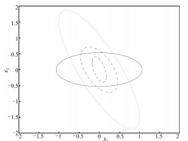
The terminal regions X0 obtained by the proposed method (solid line) and the LQR method with J1(x)
(dashed line), J2(x) (dash-dotted line) and J3(x) (dotted line).
 Volume 4
Issue 3
Volume 4
Issue 3
IEEE/CAA Journal of Automatica Sinica
| Citation: | Defeng He, "Dual-mode Nonlinear MPC via Terminal Control Laws With Free-parameters," IEEE/CAA J. Autom. Sinica, vol. 4, no. 3, pp. 526-533, July 2017. doi: 10.1109/JAS.2016.7510013

|
Nonlinear model predictive control (NMPC) has received great attentions in both academic and industrial communities [1]-[4]. The attentions of NMPC are motivated by its advantages for control of multivariable nonlinear systems and for explicitly handling constraints on process variables. Due to using the receding horizon principle, in general the closed-loop stability of NMPC cannot be guaranteed automatically by itself. To address this stability issue, many schemes have been proposed to achieve the closed-loop stability of NMPC for the last two decades [1]-[4]. One of main schemes used to ensure the closed-loop stability of NMPC is the dual-mode strategy [5]-[10], in which the MPC law is parameterized with a fixed state feedback computed offline (often called terminal controllers) and then, additional corrections are computed online. By the additional corrections, the closed-loop states are steered into an invariant set (often called terminal domain) corresponding to the feedback law computed offline. Therefore, not only most of the heavy computations related to invariance and feasibility constraints are handled offline, but also the closed-loop stability of NMPC is ensured by exploiting the feedback law computed offline.
In dual-mode NMPC schemes, the size of the maximal feasible invariant set (denoted XN) is dependent on the terminal region (denoted X0), the terminal controller ul(x) and the prediction horizon N. In general, the terminal region X0 with larger size increases the size of the feasible set XN. However, it is difficult to obtain the quantitative interplay between each other. Hence, in the conventional dual-mode NMPC schemes [5]-[10] the closed-loop states will be driven into a predesigned X0 within or less than N steps, where a linear terminal control law ul(x)=Kx is used and is required to satisfy system constraints. For simplicity of designing controllers, the terminal law ul(x)=Kx in most dual-mode MPC schemes is usually selected as a linear quadratic optimal control law. Due to the invariance of the gain matrix K, the size of X0 may be greatly small if prediction horizon N is given. Note that the size of X0 can be extended by increasing horizon N, but this approach increases the computational demand of solving the optimization problem of NMPC online. The region X0 with a small size will decrease the size of the initial feasible set XN [1], [2], [4], which makes the performances of the dual-mode NMPC become more conservative.
In order to enlarge the size of the set XN, a straightforward method is to lengthen horizon N. However, a long N will increase the computational demand of MPC since it requires satisfying a bigger optimization problem than the one with a short N. Hence, the authors in [11]-[13] employed the notion of equilibrium surface and the scheduling method to propose the dual-mode NMPC schemes with enlarged terminal regions, where several terminal subsets are defined based on the equilibrium surface. Another method in [14] was proposed for linear systems, where the horizon N in the MPC problem was divided into prediction horizon Np and control horizon Nc and a new control mode was defined over time interval [Nc,Np]. Then there exist three control modes, i.e., the terminal law ul(x) in X0, MPC law um(x) out of X0 and new control law us(x) within [Nc,Np] and out of X0. This change enlarges the size of the terminal region and decreases the conservativeness of MPC. Now this strategy is named as the triple-mode MPC scheme and has been extended to analyze and design robust MPC of uncertain linear systems.
In this paper we consider continuous-time nonlinear systems subject to state and control constraints and propose a stabilizing dual-mode NMPC scheme using terminal control laws with free-parameters. The local control Lyapunov functions (CLFs) [15] for nonlinear systems are used to design the terminal controller with some free-parameters. Then a set of feasible parameters is selected to estimate the size of the terminal region X0 as large as possible. When the state belongs to X0, an optimal control problem is formulated to online compute the free-parameters, which leads to the optimality of ul(x) with respect to given cost functions. Conversely, a correction term is computed online when the state is out of X0. By the stability results of the general dual-mode NMPC framework, the equilibrium point of the closed-loop system with NMPC controller proposed here is shown to be asymptotically stable. Finally the numerical example of a spring-cart system [16] is considered and the presented controller is compared with the dual-mode NMPC with quadratic optimal terminal control law in terms of performance and terminal regions.
The contribution of the paper is to present a closed-loop dual-mode NMPC scheme where the terminal controller is updated using the current state at each sampling time and the size of the terminal region is decoupled from the local optimality of the terminal controller. The terminal controller and the terminal region have interplay in conventional dual-mode NMPC schemes. Hence, it is hoped that the proposed scheme provides a more convenient way than the conventional ones in terms of application. It is noted that the design of the terminal controller is motivated by the results in [17].
Consider an input-affine nonlinear system described by
| ˙x(t)=f(x(t))+g(x(t))u(t) ∀t≥0 | (1) |
where x∈Rn is the state variable, u∈Rm is the control variable, f(x) and g(x) are continuous functions in some neighborhood regions of the origin. The system is subject to the constraints on the state and control
| x(t)∈X, u(t)∈U ∀t≥0 | (2) |
where X∈Rn and U∈Rm are compact and convex sets containing the origin in their interior. It is assumed that the origin is the equilibrium point of the system and the solutions to the system (1) exist and are continuous for any initial state x(0) ∈ X and piecewise, right-continuous input u(⋅)∈U. We also assume that the states can be measured at each time instant.
Definition 1 [18]: Consider set S⊆Rn and controller u: S→U. The set S is called a positively invariant set of the system (1) in closed-loop with u(x) if its solutions x(t;x(0), u(x)) ∈ S for any t≥0 and any x(0)∈S.
Definition 2 [15]: Consider the system (1) and a positive definite function V(x). If V(x) satisfies that
| LgV(x)=0⇒LfV(x)≤0 ∀x≠0 | (3) |
then V(x) is said to be a control Lyapunov function (CLF) for the system, where the Lie derivatives LfV(x)=∂V(x)∂xf(x), LgV(x)=∂V(x)∂x[g1(x),…,gm(x)] and gi(x), i=1,…,m is the ith column of matrix function g(x). Moreover, if V(x) → ∞ when ‖x‖→∞, V(x) is a global CLF of the system.
If we can construct a (global) CLF, V(x), of system (1), we have an explicit control law that stabilizes the system to the equilibrium point.
Lemma 1 [17]: Consider the system (1) and a positive definite function V(x). Let the set D=[D1,D2]×[D3,D4] with Di > 0, i=1,…,4, α(x)=LfV(x) and β(x)=LgV(x). If V(x) is a CLF of the system, then there exists a controller with free-parameters
| u(x)=h(x,μ)=−p(x,μ)β(x)T | (4) |
where two free-parameters (μ1,μ2)=μ∈D and gain
| p(x,μ)={α(x)+μ1√α(x)2+μ2‖β(x)‖4‖β(x)‖2,if β(x)≠00, if β(x)=0 |
such that the closed-loop system is asymptotically stabilized to the origin.
Note that the control law (4) gets to the standard Sontag's one if the parameter μ=(1,1). In this case, the controller has no degrees of freedom with respect to the current state information and its performance heavily relies on the selected CLF of the controlled system. Here the control law (4) has two free-parameters that have an effect on the decaying velocity of the closed-loop system [17]. Hence, one can adjust these parameters to achieve a satisfied performance of the controller while ensuring stability of the closed-loop system.
The aim of the paper is to use the control law (4) to compute a terminal region with larger size and then is to obtain a new dual-mode NMPC scheme with guaranteed recursive feasibility and stability of the obtained NMPC.
Considering the constrained system (1) and (2), we recall the general dual-mode feedback MPC controller
| uDM(x)={π(x)+v,ifx∉X0π(x),ifx∈X0 | (5) |
where X0 is the terminal region of (1), π(x) is the local optimal controller (also called terminal controller) defined in X0 and v is the additional correction term determined by solving the finite horizon optimal control problem
| minu(s) J(x(t))s.t.˙x(s)=f(x(s))+g(x(s))u(s)x(s)∈X, u(s)∈U, ∀x∈[t,t+N]x(s)|s=t=x(t), x(s)|s=t+N∈X0 | (6) |
where x(t) is the state at current time t≥0, N>0 is the prediction horizon (for simplicity, let the prediction horizon Np equal the control horizon Nc, i.e., Np=Nc=N) and J(x) is the cost function
| J(x(t)=∫t+NtL(x(s),u(s))ds | (7) |
where the stage cost L(x,u) is a positive definite function on x and is a semi-positive definite function on u. Therefore, a dual-mode MPC algorithm can be summarized as follows:
Algorithm 1:
Step 1: Set the prediction horizon N>δ, stage cost L(x,u) and a sufficiently small sampling time δ>0, and let t=0.
Step 2: Measure the state x(t) at time t. Then solve the optimization problem (6). If feasible, apply uDM(x) to system (1), go to Step 3; Otherwise, let N=N+δ, and repeat Step 2.
Step 3: Let t=t+δ and N=N−δ, go back to Step 2.
Lemma 2 [5], [7], [12]: Consider the system (1) and optimization problem (5)-(7). If the optimization problem is feasible at the initial time, the system (1) in closed-loop with (5) is then asymptotically stable in the face of constraints (2).
Remark 1: From the optimization problem (5)-(7), it is seen that the dual-mode MPC controller is related to the triplet of the terminal region X0, terminal controller π(x) and correction term v. In traditional dual-mode NMPC, the terminal controller π(x) is typically computed offline by solving linear quadratic optimal control problems. In this setting, π(x) is predefined and X0 might be considerably small. As a result, the performance (e.g., the admissible set of initial states) of the whole MPC is conservative. In what follows, we give an alternative design of the triplet using Lemma 1, which yields a new dual-mode NMPC scheme of the constrained nonlinear system (1) and (2).
In this section, we re-design the terminal region X0 and terminal controller π(x) by the assumption of the known CLF of system (1) and then propose a new dual-mode NMPC scheme for the system.
Let the function V(x) be a known, local CLF of system (1). We define a level set of V(x)
| X0(c)={x∈Rn:V(x)≤c} | (8) |
where the radius c>0. Clearly, the size of region X0 is determined by the value of c. To derive an X0 as large as possible, we define a set Xh via the terminal controller (4)
| Xh={x∈Rn:∃μ∈D s.t. h(x,μ)∈U}. | (9) |
Then we increase c from 0 until the region X0(c) approaches the set X⋂Xh to the maximal extent. In this case, let c=ˆc. Hence, there exists at least a μ such that
| h(x,μ)∈U ∀x∈X0(ˆc). | (10) |
Since X0(ˆc) is the level set of V(x), it is a positively invariant set of the system (1) in closed-loop with the controller (4) subject to the constraints (2). In the following, we present an algorithm to calculate X0(ˆc) offline.
Algorithm 2:
Step 1: Partition X near the origin into l discrete points and D into r discrete points with sufficiently large integers l>0 and r>0.
Step 2: Initialize c=∞ and let i=1.
Step 3: Compute h(xi,μj) for j=1 to r, where μj= (μj1, μj2). If h(xi,μj)∉U for all j=1,…,r, then go to Step 4; Else, go to Step 5.
Step 4: If V(xi)≤c, then let c=V(xi) and go to Step 5.
Step 5: Let i=i+1. If i≤l, then go back to Step 3; Else, go to Step 6.
Step 6: Let ˆc=c and save ˆc.
Note that the value ˆc computed by Algorithm 2 may be conservative and the computational burden is expensive due to enumeration calculation. Nevertheless, this computation process does not increase the computational burden of online solving NMPC optimization problems since it is an algorithm operated offline.
Lemma 3: Let V(x) be a known, local CLF of system (1). Then the system (1) in closed-loop with the controller (4) satisfies the constraints (2) while asymptotically stabilizing the origin in the invariant set X0(ˆc).
Proof: Since the constraint sets X and U contain the origin as their interior, the level set of V(x) exists and is non-empty. Then applying Lemma 1 directly yields Lemma 3 and hence, the proof is omitted.
Remark 2: It should be pointed out that there are no systematic methods to find a global CLF for the nonlinear systems, such as ˙x=f(x,u). For the system (1), however, the local CLF can be computed by some existing methods [15], [18]-[20], e.g., the linearization at the equilibrium points, the feedback linearization, the backsteping control, etc. In this paper, we focus on the presentation of a new dual-mode MPC scheme for system (1). Hence, it is always assumed here that a local CLF of (1) has been constructed a prior.
Remark 3: Considering the nonlinear systems with an equilibrium surface, we use the proposed approach to calculate a terminal region for every equilibrium point on the surface. Then by the gain scheduling technique, we obtain an enlarged terminal region of the whole nonlinear system. For details, see e.g. [11]-[13].
Unlike the conventional dual-mode NMPC, where the terminal controllers are typically selected as the linear quadratic regulator (LQR) controllers with the cost functions of NMPC, here we use the controller (4) as the terminal control law of the new dual-mode NMPC scheme. Note that the controller (4) has free-parameters μ1 and μ2. From [17], it is known that the parameters (μ1,μ2) are the measurement of decaying velocity of the CLF of (1). In this way, the parameters have an important effect on the control performance of the closed-loop system if the CLF is viewed as a virtual energy function of the system. Consequently, the parameters can be determined online by some additional requirements.
Here we consider the cost function (7) and define an optimal control problem
| minμ(t)∈D J(x(t))s.t.˙x(s)=f(x(s))+g(x(s))h(x(s),μ(t))x(s)∈X0(ˆc), h(x(s),μ(t))∈Ux(s)|s=t=x(t) ∀x∈[t,t+N] | (11) |
where the function h(x,μ) is given by (4) and the set X0(ˆc) is computed by (8)-(10). From the determination of ˆc, we know that there is at least a μ satisfying the constraints in problem (11), i.e., the problem is always feasible for any current state x(t) ∈ X0(ˆc).
Let μ∗(t) be an optimal solution to (11) at time t. Then the terminal control law defined in the terminal region X0(ˆc) is defined as
| π(x(t))=h(x(t),μ∗(t)). | (12) |
Note that in order to decrease the computational demand of problem (11), the parameters μ(t) are assumed to be constant within the prediction horizon window [t,t+N]. However, from the receding horizon principle we know that μ(t) at each time t is computed based on the state x(t) at the current time t. Therefore, the obtained controller (12) is a closed-loop feedback control law since the parameters are dependent upon the current state x(t).
Consider the nonlinear system (1) with constraints (2), the terminal region X0(ˆc) and terminal controller (12). We define a new dual-mode controller
| uDM(t)={h(x(t),ˆμ)+v(t),ifx(t)∉X0(ˆc)h(x(t),μ∗(t)),ifx(t)∈X0(ˆc) | (13) |
where ˆμ∈D is an offline identified number such that h(x,ˆμ) satisfies constraints (2), μ∗(t) is the optimal solution to (11) at time t and the correction term v(t) is determined by solving the finite horizon optimal control problem
| minv(s) J(x(t)) | (14) |
| s.t.˙x(s)=f(x(s))+g(x(s))[h(x(s),ˆμ(t))+v(s)]x(s)∈X, x(s)|s=t=x(t), x(s)|s=t+N∈X0(ˆc)h(x(s),ˆμ)+v(s)∈U ∀x∈[t,t+N] | (15) |
where the cost function J(x) is given by (7), function h(x,μ) is given by (4) and set X0(ˆc) is computed by (8)-(10). Then an overall dual-mode NMPC algorithm is presented below:
Algorithm 3:
Step 1: Set N>0, L(x,u) and 0<δ<N, and let t=0.
Step 2: Offline compute X0(ˆc) by (8)-(10) and pick a feasible solution ˆμ∈D.
Step 3: Measure the state x(t) at time t. If x(t)∈X0(ˆc), then solve (11) and go to Step 5. Else, solve (14). If (14) is feasible, then v(t)=v∗(t) and go to Step 4. Else, let N=N + δ and go to Step 3.
Step 4: Apply uDM(t)=h(x(t),ˆμ)+v∗(t) to system (1) and let t=t+δ and N=N−δ; go back to Step 3.
Step 5: Apply uDM(t)=h(x(t),μ∗(t)) to system (1) and let t=t+δ; go back to Step 3.
Note that the optimal control problems (11) and (14) in Algorithm 3 are nonlinear programming problems and in general, are non-convex due to the nonlinear equality constraints. Several optimization methods, such as successive quadratic programming (SQP) and genetic algorithm (GA), can be used to solve these optimization problems. Some reviews on optimization methods for solving constrained model predictive control can be consulted elsewhere, see e.g. [21], [22].
It should be pointed out that the decision variables of the optimal control problem (14) can be selected as μ and v, which increases the degrees of freedom of (14) to be optimized. However, this selection increases the computational demand of solving (14) although it may enlarge the feasible set of initial states of the controller. In addition, the effects dictated by fixing μ can be compensated to some degree by the online optimization of the correction term v.
In the sequel, we consider the optimization feasibility and stability of the dual-mode NMPC controller (13) obtained from Algorithm 3.
Definition 3: Consider a state ξ∈X of system (1). If there is a solution v(s) satisfying the problem (14) with x(s)|s=t = ξ, then ξ is said to be a feasible state. All feasible states constitute a feasible set XN of (13).
In general, we have X0⊆XN⊆X and XN⊆XN+1 for nominal system (1).
Lemma 4: Consider two positive integers N1 and N2 with N1 < N2. Then the feasible sets of (1) satisfy XN1⊆XN2.
Proof: Consider any state x(t)∈XN1 at time t. Solving the problem (14) with N=N1, we have an optimal solution v∗(s) and its associated controller u(s)=h(x(s),ˆμ)+v∗(s) for s∈[t,t+N1]. Meanwhile, the terminal state x(t+N1)∈X0(ˆc).
Let N=N2 and consider a candidate solution to (14)
| v(s)={v∗(s)∀s∈[t,t+N1]0∀s∈(t+N1,t+N2] | (16) |
which leads to an associated controller
| u(s)={h(x(s),ˆμ)+v∗(s)∀s∈[t,t+N1]h(x(s),ˆμ)∀s∈(t+N1,t+N2]. | (17) |
From Lemma 3 and the construction of the dual-mode controller (13), there exists a ˆμ∈D such that X0(ˆμ) is a positively invariant set of the constrained system (1) and (2) in closed-loop with the controller (4). Substituting (15) into the problem (14) with the initial state x(t) and the horizon N2, it is obtained that the constraints in (14) are fulfilled. This implies that the candidate (15) is a feasible solution to (14) at time t. From the Definition 3, x(t)∈XN2 and it leads to XN1⊆XN2 due to arbitrariness of x(t).
Lemma 4 implies that one can use a larger prediction horizon N to enlarge the feasible set XN, i.e., to enhance the initial feasibility. Nevertheless, the larger N generally increases the computational demand of solving the optimal control problem (14).
Theorem 1: If the optimization problem (14) is feasible at initial time t=0, then the constrained closed-loop system (1), (2) and (13) by Algorithm 3 is asymptotically stable in invariant feasible set XN. Then XN is a domain of attraction of the closed-loop system.
Proof: First from Lemma 3 and Algorithm 3, it is known that the overall dual-mode NMPC controller (13) is always feasible provided that problem (14) is initially feasible in feasible set XN. Then by Definitions 1 and 3 and Algorithm 3, we have that XN is an invariant set. Moreover, from Lemmas 2 and 3, it is obtained that the closed-loop system (1) and (13) by Algorithm 3 are asymptotically stable in XN. Therefore, all trajectories of the closed-loop system starting in XN converge to the origin. Then the invariant set XN is a domain of attraction of the closed-loop system.
Remark 4: In the dual-mode NMPC scheme presented here, some free parameters are introduced into the terminal controller π(x)=h(x,μ). An advantage of this is to decouple the local optimality of the terminal control law from the size of the terminal region. So, using a feasible set of parameters μ leads to a terminal region as large as possible while minimizing cost functions of NMPC with respect to the parameters to regain the local optimality of the terminal control law to some extent. Note that the terminal control law and the terminal region have interplay in conventional dual-mode NMPC schemes. Moreover, the terminal controller in the proposed scheme is updated based on the current state at each sampling time. In addition, the overall dual-mode NMPC controller is a state feedback control law, i.e., a closed-loop controller. This is helpful in control of uncertain systems with small disturbances.
In this section, a spring-cart is used to illustrate the performance of the results presented here, compared to the dual-mode NMPC via the LQR method. All optimization problems in this example had been solved by the fmincon function with the SQP algorithm in MATLAB 7.1 on the laptop with MS Windows XP and an Intel (R) CoreTM 2 CPU with 2.0 GHz and 1 GB RAM. The Euler's first-order approximation had been used to obtain all derivatives in this simulation.
Consider the continuous time model of the cart-spring system [16]:
| ˙x1(t)=x2(t)˙x2(t)=−kMe−x1(t)x1(t)−hMx2(t)+u(t)M | (18) |
where x1 is the displacement of the carriage from the equilibrium, x2 is the carriage velocity, u is the external force, M is the mass, k is spring elasticity and h is a damping factor. The parameters of the model are M = 1 kg, k = 0.33 and h = 1.6. Let the constraints on the state and control X=[−2,2] × [−2,2] and U=[−1,1], respectively.
Define a candidate CLF of system (17)
| V(x)=0.5x21+x22. | (19) |
It can be verified that V(x) is a CLF of (17). Then we can construct the function h(x,μ) in (4) with
| α(x)=LfV(x)=x1x2(1−4ke−x1M)−4hx22Mβ(x)=LgV(x)=4x2M. |
Compute offline a terminal region X0(ˆc) with ˆc=0.572, which is pictured as an ellipsoid denoted by solid ellipse in Fig. 1. To compare with the performance of the conventional dual-mode NMPC, we use an LQR controller based on linearized model of system (17) on the origin to compute the terminal region.
For the linearized system of (17)
| ˙x1(t)=x2(t)˙x2(t)=kMx1(t)−hMx2(t)+u(t)M | (20) |
we consider the following three quadratic stage costs
| L1(x,u)=10x21+10x22+u2 | (21) |
| L2(x,u)=x21+5x22+u2 | (22) |
| L3(x,u)=x21+x22+u2. | (23) |
Then solving the Riccati equation of system (17) with respect to L1(x,u), L2(x,u) and L3(x,u), respectively, we have three corresponding LQR controllers ui(x)=Kix for i = 1, 2 and 3 with
| P1=[14.59643.50943.50942.8248], K1=[3.50942.8248]P2=[3.91191.38301.38301.6134], K2=[1.38301.6134]P3=[3.17661.38301.38300.9152], K3=[1.28200.9152]. |
Furthermore, we compute the terminal region X0(ci) associated with Li(x) for i = 1, 2 and 3
| X0(ci)={x∈R2:xTPix≤ci}⊆{x∈X:|Kix|≤1} |
with c1=0.32, c2=0.58 and c3=1.10. These terminal regions are shown in Fig. 1, where dashed ellipse denotes X0(c1), dash-dotted ellipse X0(c2) and dotted ellipse X0(c3).
It is observed from Fig. 1 that the terminal region X0 in the proposed dual-mode NMPC scheme is independent of the cost function used while X0 in LQR-based dual-mode NMPC scheme couples with the cost function by the way of the terminal LQR controllers. Thus, in order to derive a maximal terminal region in the LQR-based dual-mode NMPC scheme, we should elaborately select the cost function (e.g., L3(x)). However, the cost function of a controlled system is usually pre-given according to some control tasks of the system. In this setting, we may have a very small terminal region (e.g., L1(x) and X0(c1)) and a corresponding small feasible state set XN for the dual-mode NMPC controller.
In order to more clearly show the differences of XN associated with X0(ci), Table Ⅰ tabulates the shortest prediction horizon Nmin that is used to guarantee the feasibility of the optimization problem (14) at initial time t0=0 with two initial states A (−1.0,1.7) and B (1.5,−1.2). It can be seen that for the different stage cost functions (20)-(22), the Nmin associated with X0(c1) is longest, the Nmin with X0(c2) is the second longest and the Nmin with X0(c3) is shortest. The reason causing this difference is due to the different size of X0(ci). This fact is also in accord with the accepted conclusion of NMPC, which inversely implies that the feasible state set XN with X0(c3) has a larger size than the other's if the prediction horizon of each controller is selected to be equal.
| Initial states | X0(ˆc) | X0(c1) | X0(c2) | X0(c3) |
| A (−1.0,1.7) | 3δ | 12δ | 3δ | δ |
| B (1.5,−1.2) | 3δ | 10δ | 5δ | 3δ |
 DownLoad:
CSV
DownLoad:
CSV
Denote by CLF-MPC and LQR-MPC the proposed dual-mode NMPC scheme and the LQR-based dual-mode NMPC scheme, respectively. We consider the stage costs Li(x,u) for i= 1, 2 and 3 and the prediction horizon N=15δ with a sampling time δ=0.25 s, and let the sector of μ be [0.1,5]×[0.1,10]. Figs. 2-4 show the state, control input and parameters (μ1,μ2) time profiles of the separate closed-loop systems starting from the initial state A, where Fig. 2 is obtained by applying L1(x,u), Fig. 3 is obtained by L2(x,u), and Fig. 4 is obtained by L3(x,u). In these figures, the solid lines are the results of CLF-MPC, the dotted lines are the results of LQR-MPC, the solid lines in right-lower subfigure are the computed parameter μ1 and the dash-dotted lines in right-lower subfigure are the computed parameter μ2. It is observed from Figs. 2-4 that:


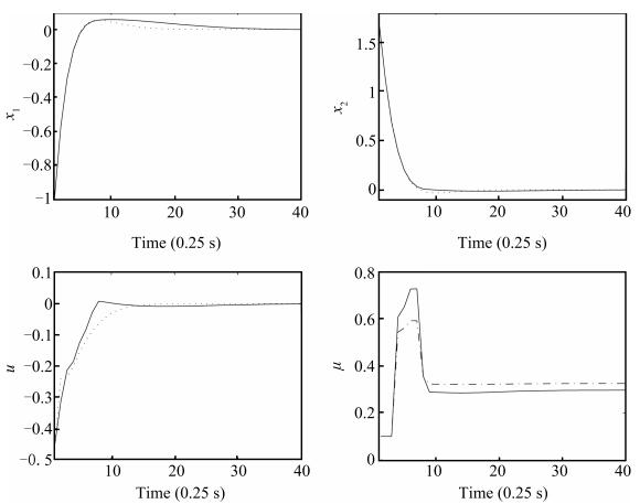
1) For any stage cost Li(x,u) for i=1,2,3, the origin of the system (15) in closed-loop with CLF-MPC is asymptotically stable while satisfying the state and control constraints.
2) Although the state trajectories obtained by CLF-MPC are similar to those by LQR-MPC, there exists an obvious difference of the control inputs obtained separately by CLF-MPC and LQR-MPC. For instance, we can see that the profiles obtained by CLF-MPC are smoother than those by LQR-MPC, which benefits the running of the controlled systems.
Table Ⅱ presents the sum of stage costs Li(x,u) over the simulation time. From Tables Ⅰ and Ⅱ, it is observed that:
| Controllers | L1(x,u) | L2(x,u) | L3(x,u) |
| CLF-MPC | 14.8126 | 6.0822 | 1.6797 |
| LQR-MPC | 14.8084 | 6.0842 | 1.6818 |
DownLoad:
CSV
1) Although the size of XN associated with X0(ˆc) is less than that with X0(c3), the performance value of L3(x,u) of CLF-MPC evaluated over the simulation time is better than that of LQR-MPC.
2) The size of XN associated with X0(ˆc) is more than that with X0(c2) and the performance value of L2(x,u) of CLF-MPC is better than that of LQR-MPC.
3) The size of XN associated with X0(ˆc) is much more than that with X0(c1), although the performance value of L1(x,u) of CLF-MPC is worse than that of LQR-MPC.
These observations imply that the CLF-MPC is better than the LQR-MPC in the terms of the feasible state set and the sum of stage costs. Note that one should elaborately select the stage cost L(x,u) in order to achieve some good performances of the feasible state set and the sum of stage costs. Hence, the proposed dual-mode NMPC presents much more flexibility and convenience than the traditional dual-mode NMPC in applications.
The paper presented a new dual-mode nonlinear model predictive control scheme for constrained continuous-time nonlinear systems. The main idea is to use control Lyapunov functions of the nonlinear system to design a terminal controller with some free-parameters and to select the parameters such that the terminal region was as large as possible. Optimality of the terminal controller was regained by optimizing the free-parameters with respect to some given cost functions. Then a varying time-horizon dual-mode NMPC scheme was proposed, whose recursive feasibility and stability were established. The example of the spring-cart system was used to demonstrate the advantages of the proposed scheme here, by comparing with the LQR-based dual-mode NMPC scheme.
Proof: Consider the system (1) and assume V(x) is a known CLF of (1). For any given parameters μ∈D, we have the derivative of V(x) along the trajectories of the system in closed-loop with the control law (4)
| ˙V(x)=α(x)+β(x)u(x)={−μ1√α(x)2+μ2β(x)4,ifβ(x)≠0α(x),ifβ(x)=0. |
From the property of CLFs, setting u≡0 leads to ˙V(x)= α(x) ≤ 0 for the state x satisfying β(x)=0. Integrating the state x satisfying β(x)≠0, we have ˙V(x)≤0 for all states.
Based on the Lyapunov's arguments, the above inequality implies that the origin of the closed-loop system is stable. Furthermore, the function V(x) satisfies that
| ˙V(x)=0 ⇔ α(x)=0, β(x)=0 |
for all states. If the closed-loop system has only trivial solution satisfying α(x)=0 and β(x)=0, then the origin is asymptotically stable according to the LaSalle's theorem [19].
| [1] |
D. Q. Mayne, J. B. Rawlings, C. V. Rao, and P. O. M. Scokaert, "Constrained model predictive control: Stability and optimality, " Automatica, vol. 36, no. 6, pp. 789-814, Jun. 2000. http://dl.acm.org/citation.cfm?id=2236626.2236892
|
| [2] |
Y. G. Xi and D. W. Li, "Fundamental philosophy and status of qualitative synthesis of model predictive control, " Acta Automat. Sin. , vol. 34, no. 10, pp. 1225-1234, Oct. 2008. http://www.oalib.com/paper/1515870
|
| [3] |
J. H. Lee, "Model predictive control: review of the three decades of development, " Int. J. Control Automat. Syst. , vol. 9, no. 3, pp. 415-424, Jun. 2011. doi: 10.1007/s12555-011-0300-6
|
| [4] |
D. F. He, B. C. Ding, and S. Y. Yu, "Review of fundamental properties and topics of model predictive control for nonlinear systems, " Control Theory Appl. , vol. 30, no. 3, pp. 273-287, Mar. 2013. https://www.researchgate.net/publication/282134530_Review_of_fundamental_properties_and_topics_of_model_predictive_control_for_nonlinear_systems
|
| [5] |
H. Michalska and D. Q. Mayne, "Robust receding horizon control of constrained nonlinear systems, " IEEE Trans. Automat. Control, vol. 38, no. 11, pp. 1623-1633, Nov. 1993. http://www.researchgate.net/publication/3021610_Robust_receding_horizon_control_of_constrained_nonlinear_systems
|
| [6] |
D. Limon, T. Alamo, and E. F. Camacho, "Enlarging the domain of attraction of MPC controllers, " Automatica, vol. 41, no. 4, pp. 629-635, Apr. 2005. http://dl.acm.org/citation.cfm?id=2239701
|
| [7] |
J. M. Bravo, T. Alamo, and E. F. Camacho, "Robust MPC of constrained discrete-time nonlinear systems based on approximated reachable sets, " Automatica, vol. 42, no. 10, pp. 1745-1751, Oct. 2006. http://dl.acm.org/citation.cfm?id=2025101
|
| [8] |
W. Al-Gherwi, H. Budman, and A. Elkamel, "A robust distributed model predictive control based on a dual-mode approach, " Comput. Chem. Eng. , vol. 50, pp. 130-138, Mar. 2013. http://www.sciencedirect.com/science/article/pii/S0098135412003560
|
| [9] |
M. Lazar, D. M. de la Peña, W. P. M. H. Heemels, and T. Alamo, "On input-to-state stability of min-max nonlinear model predictive control, " Syst. Control Lett. , vol. 57, no. 1, pp. 39-48, Jan. 2008. http://ieeexplore.ieee.org/document/1696000/
|
| [10] |
S. Hanba, "Robust nonlinear model predictive control with variable block length, " IEEE Trans. Automat. Control, vol. 54, no. 7, pp. 1618-1622, Jul. 2009. http://ieeexplore.ieee.org/document/5152965/
|
| [11] |
M. W. McConley, B. D. Appleby, M. A. Dahleh, and E. Feron, "A computationally efficient Lyapunov-based scheduling procedure for control of nonlinear systems with stability guarantees, " IEEE Trans. Automat. Control, vol. 45, no. 1, pp. 33-49, Jan. 2000. http://ieeexplore.ieee.org/xpls/abs_all.jsp?arnumber=827354
|
| [12] |
T. Zou, S. Y. Li, and B. C. Ding, "A dual-mode nonlinear model predictive control with the enlarged terminal constraint sets, " Acta Automat. Sin. , vol. 32, no. 1, pp. 21-27, Jan. 2006. http://kns.cnki.net/KCMS/detail/detail.aspx?filename=moto200601004&dbname=CJFD&dbcode=CJFQ
|
| [13] |
M. Zhao and S. Y. Li, "Dual-mode robust predictive control for nonlinear systems: a switching method between polyhedral invariant sets, " J. Syst. Sci. Math. Sci. , vol. 27, no. 3, pp. 365-377, Jun. 2007. http://en.cnki.com.cn/Article_en/CJFDTOTAL-STYS200703006.htm
|
| [14] |
L. Imsland, J. A. Rossiter, B. Pluymers, and J. Suykens, "Robust triple mode MPC, " Int. J. Control, vol. 81, no. 4, pp. 679-689, Apr. 2008. doi: 10.1080/00207170701644124
|
| [15] |
R. Sepulchre, M. Jankovic, and P. V. Kokotovic, Constructive Nonlinear Control. London, UK: Springer, 1997.
|
| [16] |
L. Magni, G. De Nicolao, R. Scattolini, and F. Allgöwer, "Robust model predictive control for nonlinear discrete-time systems, " Int. J. Robust Nonlinear Control, vol. 13, no. 3-4, pp. 229-246, Mar. -Apr. 2003. http://www.researchgate.net/publication/229884042_Robust_model_predictive_control_for_nonlinear_discretetime_systems
|
| [17] |
D. F. He, L. Yu, and X. L. Song, "Optimized-based stabilization of constrained nonlinear systems: a receding horizon approach, " Asian J. Control, vol. 16, no. 6, pp. 1693-1701, Nov. 2014. https://www.researchgate.net/publication/269265251_Optimized-Based_Stabilization_of_Constrained_Nonlinear_Systems_A_Receding_Horizon_Approach
|
| [18] |
F. Blanchini, "Set invariance in control, " Automatica, vol. 35, no. 11, pp. 1747-1767, Nov. 1999.
|
| [19] |
H. K. Khalil, Nonlinear Systems, 3rd ed. New Jersey, USA:Prentice Hall, Inc., 2002.
|
| [20] |
N. H. El-Farra and P. D. Christofides, "Bounded robust control of constrained multivariable nonlinear processes, " Chem. Eng. Sci. , vol. 58, no. 13, pp. 3025-3047, Jul. 2003. http://www.sciencedirect.com/science/article/pii/S000925090300126X
|
| [21] |
M. Cannon, "Efficient nonlinear model predictive control algorithms, " Annu. Rev. Control, vol. 28, no. 2, pp. 229-237, Dec. 2004.
|
| [22] |
H. G. Bock, M. Diehl, P. Kuhl, E. Kostina, J. P. Schiöder, and L. Wirsching, "Numerical methods for efficient and fast nonlinear model predictive control, " in Assessment and Future Directions of Nonlinear Model Predictive Control, R. Findeisen, F. Allgöwer, and L. T. Biegler, Eds. Berlin Heidelberg, Germany: Springer, 2007, pp. 163-179. http://www.springerlink.com/content/u3672863k3u70006/
|
| [1] | Shulei Zhang, Runda Jia. A Self-Healing Predictive Control Method for Discrete-Time Nonlinear Systems[J]. IEEE/CAA Journal of Automatica Sinica, 2025, 12(4): 668-682. doi: 10.1109/JAS.2024.124620 |
| [2] | Chenxi Gu, Xinli Wang, Kang Li, Xiaohong Yin, Shaoyuan Li, Lei Wang. Enhanced Tube-Based Event-Triggered Stochastic Model Predictive Control With Additive Uncertainties[J]. IEEE/CAA Journal of Automatica Sinica, 2025, 12(3): 596-605. doi: 10.1109/JAS.2024.124974 |
| [3] | Hongxing Xiong, Guangdeng Chen, Hongru Ren, Hongyi Li. Broad-Learning-System-Based Model-Free Adaptive Predictive Control for Nonlinear MASs Under DoS Attacks[J]. IEEE/CAA Journal of Automatica Sinica, 2025, 12(2): 381-393. doi: 10.1109/JAS.2024.124929 |
| [4] | Haijing Wang, Jinzhu Peng, Fangfang Zhang, Yaonan Wang. High-Order Control Barrier Function-Based Safety Control of Constrained Robotic Systems: An Augmented Dynamics Approach[J]. IEEE/CAA Journal of Automatica Sinica, 2024, 11(12): 2487-2496. doi: 10.1109/JAS.2024.124524 |
| [5] | Luigi D’Alfonso, Francesco Giannini, Giuseppe Franzè, Giuseppe Fedele, Francesco Pupo, Giancarlo Fortino. Autonomous Vehicle Platoons In Urban Road Networks: A Joint Distributed Reinforcement Learning and Model Predictive Control Approach[J]. IEEE/CAA Journal of Automatica Sinica, 2024, 11(1): 141-156. doi: 10.1109/JAS.2023.123705 |
| [6] | Xiongbo Wan, Chaoling Zhang, Fan Wei, Chuan-Ke Zhang, Min Wu. Hybrid Dynamic Variables-Dependent Event-Triggered Fuzzy Model Predictive Control[J]. IEEE/CAA Journal of Automatica Sinica, 2024, 11(3): 723-733. doi: 10.1109/JAS.2023.123957 |
| [7] | Yuhan Zhang, Zidong Wang, Lei Zou, Yun Chen, Guoping Lu. Ultimately Bounded Output Feedback Control for Networked Nonlinear Systems With Unreliable Communication Channel: A Buffer-Aided Strategy[J]. IEEE/CAA Journal of Automatica Sinica, 2024, 11(7): 1566-1578. doi: 10.1109/JAS.2024.124314 |
| [8] | Bing Zhu, Xiaozhuoer Yuan, Li Dai, Zhiwen Qiang. Finite-Time Stabilization for Constrained Discrete-time Systems by Using Model Predictive Control[J]. IEEE/CAA Journal of Automatica Sinica, 2024, 11(7): 1656-1666. doi: 10.1109/JAS.2024.124212 |
| [9] | Zewei Zheng, Jiazhe Li, Zhiyuan Guan, Zongyu Zuo. Constrained Moving Path Following Control for UAV With Robust Control Barrier Function[J]. IEEE/CAA Journal of Automatica Sinica, 2023, 10(7): 1557-1570. doi: 10.1109/JAS.2023.123573 |
| [10] | Wei Lu, Jiacheng Li, Huanhuan Qin, Lei Shu, Aiguo Song. On Dual-Mode Driving Control Method for a Novel Unmanned Tractor With High Safety and Reliability[J]. IEEE/CAA Journal of Automatica Sinica, 2023, 10(1): 254-271. doi: 10.1109/JAS.2023.123072 |
| [11] | Lingzhi Wang, Guo Xie, Fucai Qian, Jun Liu, Kun Zhang. A Novel PDF Shape Control Approach for Nonlinear Stochastic Systems[J]. IEEE/CAA Journal of Automatica Sinica, 2022, 9(8): 1490-1498. doi: 10.1109/JAS.2022.105755 |
| [12] | Yuzhen Liu, Ziyang Meng, Yao Zou, Ming Cao. Visual Object Tracking and Servoing Control of a Nano-Scale Quadrotor: System, Algorithms, and Experiments[J]. IEEE/CAA Journal of Automatica Sinica, 2021, 8(2): 344-360. doi: 10.1109/JAS.2020.1003530 |
| [13] | Lei Liu, Tingting Gao, Yan-Jun Liu, Shaocheng Tong. Time-Varying Asymmetrical BLFs Based Adaptive Finite-Time Neural Control of Nonlinear Systems With Full State Constraints[J]. IEEE/CAA Journal of Automatica Sinica, 2020, 7(5): 1335-1343. doi: 10.1109/JAS.2020.1003213 |
| [14] | Yu Cao, Jian Huang. Neural-Network-Based Nonlinear Model Predictive Tracking Control of a Pneumatic Muscle Actuator-Driven Exoskeleton[J]. IEEE/CAA Journal of Automatica Sinica, 2020, 7(6): 1478-1488. doi: 10.1109/JAS.2020.1003351 |
| [15] | Magdi S. Mahmoud, Mojeed O. Oyedeji. Adaptive and Predictive Control Strategies for Wind Turbine Systems: A Survey[J]. IEEE/CAA Journal of Automatica Sinica, 2019, 6(2): 364-378. doi: 10.1109/JAS.2019.1911375 |
| [16] | Bao-Lin Ye, Weimin Wu, Keyu Ruan, Lingxi Li, Tehuan Chen, Huimin Gao, Yaobin Chen. A Survey of Model Predictive Control Methods for Traffic Signal Control[J]. IEEE/CAA Journal of Automatica Sinica, 2019, 6(3): 623-640. doi: 10.1109/JAS.2019.1911471 |
| [17] | Zaiyu Chen, Minghui Yin, Lianjun Zhou, Yaping Xia, Jiankun Liu, Yun Zou. Variable Parameter Nonlinear Control for Maximum Power Point Tracking Considering Mitigation of Drive-train Load[J]. IEEE/CAA Journal of Automatica Sinica, 2017, 4(2): 252-259. doi: 10.1109/JAS.2017.7510520 |
| [18] | Yan Song, Haifeng Lou, Shuai Liu. Distributed Model Predictive Control with Actuator Saturation for Markovian Jump Linear System[J]. IEEE/CAA Journal of Automatica Sinica, 2015, 2(4): 374-381. |
| [19] | Xiaohua Xia, Jiangfeng Zhang. Operation Efficiency Optimisation Modelling and Application of Model Predictive Control[J]. IEEE/CAA Journal of Automatica Sinica, 2015, 2(2): 166-172. |
| [20] | Jing Na, Guido Herrmann. Online Adaptive Approximate Optimal Tracking Control with Simplified Dual Approximation Structure for Continuous-time Unknown Nonlinear Systems[J]. IEEE/CAA Journal of Automatica Sinica, 2014, 1(4): 412-422. |

Figures(4) / Tables(2)


Defeng He, "Dual-mode Nonlinear MPC via Terminal Control Laws With Free-parameters," IEEE/CAA J. Autom. Sinica, vol. 4, no. 3, pp. 526-533, July 2017. doi: 10.1109/JAS.2016.7510013
| Initial states | X0(ˆc) | X0(c1) | X0(c2) | X0(c3) |
| A (−1.0,1.7) | 3δ | 12δ | 3δ | δ |
| B (1.5,−1.2) | 3δ | 10δ | 5δ | 3δ |
DownLoad:
CSV
| Controllers | L1(x,u) | L2(x,u) | L3(x,u) |
| CLF-MPC | 14.8126 | 6.0822 | 1.6797 |
| LQR-MPC | 14.8084 | 6.0842 | 1.6818 |
DownLoad:
CSV
 DownLoad:

 DownLoad:


