


Figure
1.
The illustration of proposed controlled pendulum system (15).
 Volume 12
Issue 4
Volume 12
Issue 4
IEEE/CAA Journal of Automatica Sinica
| Citation: | Y. Wang and H. Li, “Global stabilization via adaptive event-triggered output feedback for nonlinear systems with unknown measurement sensitivity,” IEEE/CAA J. Autom. Sinica, vol. 12, no. 4, pp. 833–835, Apr. 2025. doi: 10.1109/JAS.2023.123984

|
Dear Editor,
This letter investigates global stabilization of uncertain nonlinear systems via adaptive event-triggered output feedback. Uncertainties lie in both system nonlinearities and measurement sensitivity. To this end, a dynamic high gain is introduced to cope with the influence of large uncertainties, the unknown measurement sensitivity and the execution error, while a time-varying threshold event-triggering mechanism is constructed to effectively exclude the Zeno phenomenon. As such, the adaptive event-triggered control ensures globally bounded and convergent of system states. The design method is demonstrated using a controlled pendulum example.
Event-triggered control has become popular over the past 20 years for improving feedback ability and saving resources in large-scale networks and distributed control. Researchers continue to develop better triggering mechanisms and expanding broader adaptation scenarios, e.g., dynamic event-triggering mechanism [1], adaptive event-triggering mechanism [2], [3], intelligent transportation [4].
Nonlinear systems are commonly affected by uncertainties, including parameter uncertainties and external disturbances [5], which could be suppressed by feedback control. While due to limitations in measurement technology and tooling accuracy, sensor sensitivity is sometimes unknown in real-world scenarios, which poses a new challenge for nonlinear system control. Recent studies propose some methods to address this issue, including a dual-domination approach [6], non-identifier based upon output-feedback control [7], combining tangent-type barrier Lyapunov function and Nussbaum-type function [8], time-varying gain for feedforward nonlinear systems [9], fuzzy logic systems for stochastic nonlinear multiagent systems [10]. Nonetheless, these methods may have some limitations, such as requiring additional information on system nonlinearities [8], the inability to guarantee the boundedness of the gain [9], or being limited to a local objective rather than a global one [10]. Therefore, how to design appropriate adaptive compensation when large uncertainties, unknown sensitivity and execution error coexist, and how to exclude the Zeno phenomenon under the influence of the unmeasurable states, have become difficult and interesting problems, on which, to our knowledge, there are few reports.
Motivated by the aforementioned, this letter studies the global stabilization of nonlinear systems through adaptive event-triggered output feedback in the presence of large uncertainties and unknown measurement sensitivity coupling to unmeasurable states. The innovative contributions of this letter focus on the following two aspects.
1) The coexistence of large uncertainties and unknown measurement sensitivity renders the event-triggered feedback design challenging. To address this, it is commended a dynamic high gain that can be adequately large to be effective while remains bounded. However, in [11], merely weak uncertainties are allowed due to lacking compensating mechanisms, while in [9], the gain signal is time-varying and would tend towards infinity as time goes on.
2) A time-varying threshold event-triggering mechanism is constructed to avoid the Zeno phenomenon effectively. The threshold is strictly positive but decays to zero, ensuring control feasibility and global convergence of system states to zero. Reference [12] merely ensures boundedness of system states because the threshold owns a positive constant lower bound, while [10] achieves a semi-global objective.
Problem statement: Consider nonlinear system as
| {˙xi=xi+1+gi(t,x),i=1,…,n−1˙xn=u+gn(t,x)y=θ1x1 | (1) |
where x=[x1,…,xn]T∈Rn is the system state equipped with x(0)=x0; u∈R is the control input; y∈R is the system output; unknown constant θ1∈R+ represents the measurement sensitivity; unknown functions gi:[0,+∞)×Rn, i=1,…,n, are locally Lipschitz and continuous in x and t, respectively.
Assumption 1: There is an unknown constant θ2∈R+ that satisfies |gi(x,u,t)|≤θ2(|y|+∑ij=2|xj|), i=1,…,n.
Assumption 2: There exist two known positive constants ˉθ and θ_, such that 0<θ_≤θ1≤ˉθ.
Remark 1: Assumption 1 implies that system (1) allows large uncertainties while the nonlinearities depend strongly on the unmeasurable states. Assumption 2 means that the measurement sensitivity is unknown. The two pose new challenges and promote the birth of the following improved event-triggered output-feedback control schemes.
Event-triggered control design: First, to rebuild the unmeasurable states in system (1), construct a high-gain state observer as
| {˙ˆxi=ˆxi+1−Liaiˆx1,i=1,…,n−1˙ˆxn=u−Lnanˆx1 | (2) |
where design parameters ai∈R+, and gain L satisfies updating law
| ˙L=(yL)2+n∑i=2(ˆxiLi)2,L(0)=1. | (3) |
It follows from (3) that dynamic gain L(t)≥1 is nondecreasing, which shows that L could be as large as enough to deal with system uncertainties and unknown measurement sensitivity. Notably, gain L is online adjusted, which means that once the initial value is given, L would evolve automatically according to the system behavior.
Then the adaptive event-triggered controller based on the emulation approach is designed as
| {u(t)=ω(tk),t∈[tk,tk+1)ω(L,ˆx,y)=−βnLn+1ηn | (4) |
where ω(L(t),ˆx(t),y(t)) is abbreviated as ω(t) following the design process in [7]. The times tk’s, i.e., the ones on which execution occurs, are yielded recursively from event-triggering mechanism as
| tk+1=inf{t>tk||δ(tk)|>e−αt} | (5) |
with δ(tk)=ω(t)−ω(tk), initial time t1=0 and pre-specified positive constant α. Define scaling transformation
| zi=ˆxiLi,εi=xi−ˆxiLi,i=1,…,n. | (6) |
Denote z=[z1,…,zn]T and ε=[ε1,…,εn]T. Then, (1)–(3) imply
| {D+z=−LβnηnC+LAz−˙LLDz+u−ωLnCD+ε=−˙LL+LAε+1θ1ay+˜g | (7) |
where A=[−a[In−10n−1]T] with a=[a1,…,an]T, C=[0,…,0,1]T, D=diag{1,…,n}, and ˜g=[g1L,…,gnLn]T. Design parameters ai’s can suitably be selected such that A is Hurwitz; there is a positive definite symmetric P such that
| ATP+PA≤−I,DP+PD≥0. | (8) |
From Lemma 1 in [13], it follows that the selection of parameters ai’s can always be achievable.
Consider the following scaling transformation and candidate Lyapunov functions similar to those in [7]:
| η1=yL,ηi=ˆxi−ˆx∗iLi,V1=12r1η21,Vi=Vi−1+η2i2ri | (9) |
where ˆx∗i=−βi−1Liηi−1, β1=1θ_(2‖, \beta_i = r_i(b_i+n) , r_i = \frac{n(i-1)(n-i+2)\prod_{k = 1}^{i-1}\beta_k^2}{4i}r_{i-1} , b_1 = \frac{3}{4}\bar\theta^2 , b_i>0 are suitable constants, and i = 2,\ldots,n . Then, the following proposition describes the dynamic evolution. The detailed proof is omitted here since it can be obtained by a simple calculation.
Proposition 1: Choose candidate Lyapunov functions V_z = z^{T} P z and V_\varepsilon = \varepsilon^{T} P\varepsilon . Then, it follows:
| \begin{equation*} \left\{ \begin{aligned} &D^+V_z\leq-\frac{L}{2}\|z\|^2+4\beta_n^2\|PC\|^2L\eta_n^2+\frac{4\|PC\|^2}{L^{2n+1}e^{2\alpha t}} \cr &D^+V_\varepsilon\leq-\Big(\frac{L}{2}-\Theta_1\Big)\|\varepsilon\|^2+n\theta_2\|P\|\times\|z\|^2 +\frac{2\|Pa\|^2L}{\theta_1^2}\Big(\frac{|y|}{L}\Big)^2 \end{aligned} \right. \end{equation*} |
in which the upper right-hand derivative of V is represented by D^+V while \Theta_1>0 is unknown.
Main results: As the similar discussion in [2], it can be deduced that, the solution (x,\hat x,L) exists, and is unique on the maximum interval [0,T_m) for any initial condition (x_0,\hat x_0) .
Proposition 2: The boundedness of gain L(t) suggests that both z(t) and \varepsilon(t) are bounded on interval [0,T_m) , as well as
| \begin{eqnarray*} \lim_{t\to T_m}\int_0^{t}\Big(\|\varepsilon(s)\|^2+\|z(s)\|^2\Big) {{d}} s < +\infty. \end{eqnarray*} |
Proof: It follows from the boundedness of the gain that \bar L = \sup_{t\in[0,T_m)}L(t) = \lim_{t\to T_m}L(t) , for some positive constant \bar{L} .
1) z(t) is bounded and quadratic integrable for any t\in[0,T_m) .
From Proposition 1, one has
| \begin{equation*} D^+V_z \leq-\frac{L}{2}\|z\|^2+4\beta_n^2\|PC\|^2L\eta_n^2+\frac{4\|PC\|^2}{L^{2n+1}e^{2\alpha t}}. \end{equation*} |
From the definition of \hat x_i^* and \eta_i , it can be recursively derived \hat x_n^* = -\sum_{i = 1}^{n-2}\left(\prod_{j = 1}^i\beta_{n-j}\right)L^i\hat x_{n-i}-\left(\prod_{i = 1}^{n-1}\beta_i\right)L^{n-1}y , which combining with (9) implies \eta_n^2 \leq M\big(\frac{y}{L}\big)^2+M\sum_{i = 2}^n\big(\frac{\hat x_i}{L^i}\big)^2 = M\dot L , where M = \max\big\{n,n\big(\prod_{j = 1}^i\beta_{n-j}\big)^2,n\big(\prod_{k = 1}^{n-1}\beta_k\big)^2\big\} , i = 1,\ldots,n-2 . Then, by the hypothesis and noting L\geq1 and V_z = z^{T} P z , there holds
| \begin{equation} D^+V_z \leq-\lambda V_z+4\|PC\|^2\beta_n^2\bar L\dot L+\frac{4\|PC\|^2}{e^{2\alpha t}} \end{equation} | (10) |
with \lambda = \frac{1}{2\lambda_{\max(P)}} , which is equivalent to
| \begin{equation*} D^+\big(e^{\lambda t}V_z\big) \leq 4\beta_n^2\|PC\|^2\bar Le^{\lambda t}\dot L+4\|PC\|^2e^{\lambda t}. \end{equation*} |
Then, for \forall t\in[0,T_m) we get V_z(t) \leq 4 \|PC\|^2\beta_n^2\bar L^2+\frac{4\|PC\|^2}{\lambda} , which indicates that z(t) maintains bounded on interval [0,T_m) . Integrating (10) from 0 to t, \forall t\in[0,T_m) , we obtain V_z(t)-V_z(0) \leq- \lambda \int_{0}^{t} V_z(s){d}s +4 \|PC\|^2\beta_n^2\bar L \int_{0}^{t} \dot L(s){d} s +4\|PC\|^2 \int_{0}^{t} \frac{1}{e^{2\alpha s}}{d}s, which derives
| \begin{eqnarray*} \lambda \int_{0}^{t} V_z(s){d}s \leq 4\beta_n^2\|PC\|^2\bar L^2+\frac{2\|PC\|^2}{\alpha}+V_z(0)<+\infty. \end{eqnarray*} |
Then, from V_z = z^{T} Pz , one gets \lim_{t\to T_m}\int_0^{t}\|z(s)\|^2{d}s<+\infty .
2) \varepsilon(t) is bounded and quadratic integrable for any t\in[0,T_m) .
Construct scaling observer error
| \begin{eqnarray} \xi_i = \frac{x_i-\hat{x}_i}{(L^*)^i}, \quad i = 1,\ldots,n \end{eqnarray} | (11) |
with a design parameter L^* . Let \xi = [\xi_1,\ldots,\xi_n]^{T} . Then, (1), (2) and (11) imply \dot\xi = L^*A\xi+L^*a\xi_1-L\Lambda a\xi_1+\frac{1}{\theta_1}L\Lambda a\frac{y}{L^*}+\tilde g^* with \tilde g^* = \big[\frac{g_1}{L^*},\ldots, \frac{g_n}{(L^*)^n}\big]^{T} and \Lambda = {{\rm{diag}}}\big\{1,\frac{L}{L^*},\ldots,(\frac{L}{L^*})^{n-1}\big\} . Derivate the candidate Lyapunov function V_\xi = \xi^{T} P\xi . One obtains
| \begin{split} D^+V_\xi =\; & L^*\xi^{T}(A^{T} P+PA)\xi+2L^*\xi_1\xi^{T} P a-2L\xi_1\xi^{T} P\Lambda a\nonumber\cr & +\frac{2}{\theta_1}L\xi^{T}P\Lambda a\frac{y}{L^*}+2\xi^{T} P\tilde g^*. \end{split} |
Similar to the treatment of Proposition 1, it can be deduced that
| \begin{align*} D^+V_\xi &\leq -(L^*-\Theta_2)\|\xi\|^2+c_1\left(\frac{|y|}{L}\right)^2 +c_2\sum\limits_{i = 2}^n\left(\frac{\hat x_i}{L^i}\right)^2 \end{align*} |
with c_1 , c_2 and \Theta_2 being some positive constant. This, together with the choice of L^* ( L^*>\max\{\Theta_2+1,\bar L\} ) and (3), suggests that
| \begin{align} D^+V_\xi &\leq -2\lambda V_\xi+\max\{c_1,c_2\}\dot L. \end{align} | (12) |
Then, we get V_{\xi}(t) \leq \max\{c_1,c_2\}\bar L , \forall t\in[0,T_m) , which says that \xi(t) keeps bounded on [0,T_m) . Noting \varepsilon_i = \frac{L^*}{L}\xi_i and the boundedness of L, it is clear that \varepsilon(t) stands bounded on [0,T_m) . For any t\in [0,T_m) , integrate (12) from 0 to t. Then one obtains V_\xi(t)-V_\xi(0) \leq -2\lambda\int_0^{t}V_\xi(s){d}s+\max\{c_1,c_2\}\bar L, which yields
| \begin{eqnarray*} 2\lambda\int_0^{t}V_\xi(s){d}s \leq V_\xi(0)+\max\{c_1,c_2\}\bar L<+\infty. \end{eqnarray*} |
Thus, by V_{\xi} = \xi^{T} P\xi , it can be derived \lim_{t\to T_m}\int_0^{t}\|\xi(s)\|^2{d}s<+\infty . Noting \varepsilon_i = \frac{L^*}{L}\xi_i and the boundedness of L again, one sees that \lim_{t\to T_m}\int_0^{t}\|\varepsilon(s)\|^2{d}s < +\infty.
Proposition 3: The boundedness of all resulting closed-loop signals means T_m = +\infty and no Zeno phenomenon occurs. Besides, as t tends to infinity, (x(t),\hat x(t),u(t)) tends to zero.
Proof: By contradiction, suppose T_m<+\infty . Together with the boundedness of the closed-loop signals, it indicates that Zeno occurs, i.e., there exists an infinite time sequence \{t_k\} ’s in [0,T_m) such that \lim_{k\to+\infty}t_k = T_m .
Note the boundedness of the signals, which, together with (2)–(5), implies the existence of a constant M>0 such that \big|D^+\big(e^{2\alpha t}(u(t)- \omega(t))^2\big)\big|\nonumber \; \leq\; 2\big|u(t)-\omega(t)\big|\cdot\big|D^+\omega(t)\big|e^{2\alpha t}+2\alpha \big(u(t)-\omega(t)\big)^2e^{2\alpha t} \; \leq\; Me^{\alpha t}. Then, we have
| \begin{equation} \lim\limits_{t\rightarrow t_{k+1}} \int_{t_k}^t D^+\big(e^{2\alpha s}(u(\tau)-\omega(s))^2\big){d}s \leq \frac{M}{\alpha}\big(e^{\alpha t_{k+1}}-e^{\alpha t_k}\big). \end{equation} | (13) |
On the other hand, according to event-triggering mechanism (5),
| \begin{equation*} 1 = \lim\limits_{t\rightarrow t_{k+1}}\big(u(t)-\omega(t)\big)^2e^{2\alpha t} -\big(u(t_k)-\omega(t_k)\big)^2e^{2\alpha t_k} \end{equation*} |
which together with (13), means 1\leq\frac{M}{\alpha}\big(e^{\alpha t_{k+1}}-e^{\alpha t_k}\big) . Then, Lagrange mean value theorem implies the existence of \beta_k\in[t_k,t_{k+1}) such that Me^{\alpha\beta_k}(t_{k+1}-t_k)\geq 1 , i.e., t_{k+1}-t_k\geq\frac{1}{Me^{\alpha\beta_k}}>\frac{1}{Me^{\alpha T_m}}>0 since T_m< +\infty . However, from this, it follows \lim_{k\to+\infty}t_k = +\infty , which is a contradiction. Thus, we conclude T_m = +\infty and there is no Zeno phenomenon.
It remains to prove that system states and control signal converge to zero. Since the closed-loop signals are bounded, which, together with (7), suggests D^+z and D^+\varepsilon hold boundedness on [0,+\infty) . Additionally, Proposition 2 indicates
| \begin{eqnarray*} \lim_{t\to+\infty}\int_0^{t}(\|\varepsilon(s)\|^2+\|z(s)\|^2){d} s < +\infty. \end{eqnarray*} |
Then, one obtains \lim_{t\to+\infty}(\varepsilon(t),z(t)) = (0,0) from Barbălat Lemma [14]. Combining (6) with L(t)\geq1 , it holds that \lim_{t\to+\infty}(x(t),\hat{x}(t)) = (0,0) . Since on interval [0,+\infty) , all closed-loop signals keep bounded, which, together with (4) and (9), implies \lim_{t\to+\infty}u(t) = 0 .
The following theorem summarizes the main result of this letter, which establishes the conditions for the closed-loop signals to be bounded and convergent on the existence interval of the solution.
Theorem 1: With Assumptions 1 and 2 imposed on system (1), design output feedback control (4) under event-triggering mechanism (5), combined with state observer (2) and dynamic high gain (3). Then, the resulting closed-loop system is globally bounded while \lim_{t\to+\infty}(x(t),\hat x(t),u(t)) = (0,0,0) . Besides, the Zeno phenomenon does not occur.
Proof: For any (x_0,\hat x_0) , as mentioned at the beginning of this part, the unique solution exists on [0,T_m) .
From Propositions 2 and 3, it follows that to finish the proof of the theorem, we only need to verify that gain L(t) remains bounded on [0,T_m) . Contradictory, assume that L(t) can be unbounded on [0,T_m) . Then, from the nondecreasing property of the gain, one obtains \lim_{t\to T_m}L(t) = +\infty , which suggests the existence of T_1\in(0,T_m) such that L(t)\geq\Theta_3, \forall t\in[T_1,T_m) for some \Theta_3 .
Take candidate Lyapunov function as V = (n+1)V_{\varepsilon}+V_n . Then, with similar to the process of (48) in [7], we get
| \begin{eqnarray} D^+V\leq-\|\varepsilon\|^2-\|\eta\|^2, \quad \forall t\in[T_1, T_m). \end{eqnarray} | (14) |
On the other hand, \dot L = \eta_1^2+\sum_{i = 2}^n(\eta_i-\beta_{i-1}\eta_{i-1})^2\leq\bar\beta\|\eta\|^2 , which, together with (14), indicates that
| \begin{align*} +\infty & = L(T_m)-L(T_1) = \int_{T_1}^{T_m}\dot Ldt \leq \int_{T_1}^{T_m}\bar\beta\|\eta\|^2dt \nonumber \cr &\leq \bar\beta V(T_1) <+\infty. \end{align*} |
The contradiction shows that L(t) must be bounded on [0,T_m) .
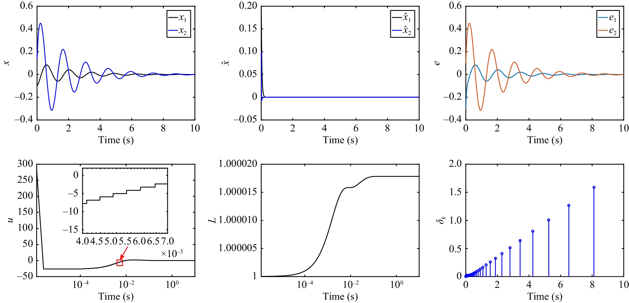
Numerical example: A controlled pendulum system in the following form is considered to illustrate the effectiveness of our design approach above:
| \begin{equation} \left\{ \begin{aligned} &\dot{x}_1 = x_2\cr &\dot{x}_2 = u-mg\sin\frac{x_1}{ml}-\frac{k}{m}x_2\cr &y = \theta x_1. \end{aligned} \right. \end{equation} | (15) |
Parameters m and l represent mass and length, respectively, g denotes gravitational acceleration and k is the friction coefficient, which is commonly an unknown constant.
Assume that 1.25\leq\theta\leq1.3 . Obviously, pendulum system (15) satisfies Assumptions 1 and 2. Let m = 2 , l = 0.5 , k = 2 and g = 9.8 . Put the initial system states as [-0.1,0.2]^{T} and the initial observer states as [0.2,0.1]^{T} . Select the design parameters in observer (2) as a_1 = 25 , a_2 = 17 . Solve inequality (8) and we obtain P = \big[ \begin{smallmatrix} \; \; 0.5389 & -0.7109 \cr -0.7109 & \; \; 1.0764 \end{smallmatrix} \big]. Thus, following the previous design process, \frac{2\|Pa\|^2}{\underline\theta^2} = 2.82 , b_1 = 1.27 , \beta_1 = 9.39 , r_2 = 44.06 , b_2 = 3.93 . Hereinto, the parameter in event-triggering mechanism (5) is selected as \alpha = 1 . By utilizing MATLAB, one obtains the system evolution shown in Fig. 1. As such, the designed event-triggered control makes system states stay bounded and convergent to zero, and no Zeno phenomenon occurs.
Conclusion: Global event-triggered stabilization of nonlinear systems is addressed for uncertainties in both system nonlinearities and measurement sensitivity. For this purpose, a new design for the state observer and dynamic high gain is conducted by utilizing the system output and observer states. An effective event-triggered control in the case of output feedback is proposed by introducing certain auxiliary parameters. It synthesizes the implications of large uncertainties, unknown output, and the execution error to guarantee global stabilization. Future work might be directed towards more general systems such as those with polynomial-of-output growth.
Acknowledgments: This work was supported by the National Natural Science Foundation of China (62203283), Shandong Provincial Natural Science Foundation (ZR2022QF009, ZR2023QA063), and the China Postdoctoral Science Foundation (2022M711981).
| [1] |
A. Girard, “Dynamic triggering mechanisms for event-triggered control,” IEEE Trans. Autom. Control, vol. 60, no. 7, pp. 1992–1997, 2015. doi: 10.1109/TAC.2014.2366855
|
| [2] |
F. Li and Y. Liu, “Adaptive event-triggered output-feedback controller for uncertain nonlinear systems,” Automatica, vol. 117, p. 109006, 2020. doi: 10.1016/j.automatica.2020.109006
|
| [3] |
H. Li, Y. Liu, and F. Li, “Adaptive event-triggered output feedback for nonlinear systems with unknown polynomial-of-output growth rate,” IEEE Trans. Circuits Syst. I, vol. 69, no. 5, pp. 2179–2192, 2022. doi: 10.1109/TCSI.2022.3150434
|
| [4] |
X. Ge, S. Xiao, Q.-L. Han, X. Zhang, and D. Ding, “Dynamic event-triggered scheduling and platooning control co-design for automated vehicles over vehicular ad-hoc networks,” IEEE/CAA J. Autom. Sinica, vol. 9, no. 1, pp. 31–46, 2022. doi: 10.1109/JAS.2021.1004060
|
| [5] |
A. Prasov and H. Khalil, “A nonlinear high-gain observer for systems with measurement noise in a feedback control framework,” IEEE Trans. Autom. Control, vol. 58, no. 3, pp. 569–580, 2013. doi: 10.1109/TAC.2012.2218063
|
| [6] |
C. Chen, C. Qian, Z. Sun, and Y. Liang, “Global output-feedback stabilization of a class of nonlinear systems with unknown measurement sensitivity,” IEEE Trans. Autom. Control, vol. 63, no. 7, pp. 2212–2217, 2018. doi: 10.1109/TAC.2017.2759274
|
| [7] |
L. Liang, X. Yan, and T. Shen, “Global output-feedback adaptive stabilization for uncertain nonlinear systems with polynomial growth nonlinearities,” Syst. Control Lett., vol. 165, p. 105269, 2022. doi: 10.1016/j.sysconle.2022.105269
|
| [8] |
R. Meng, C. Hua, K. Li, and P. Ning, “Dynamic event-triggered control for nonlinear stochastic systems with unknown measurement sensitivity,” IEEE Trans. Circuits Syst. I, vol. 70, no. 4, pp. 1710–1719, 2023. doi: 10.1109/TCSI.2022.3232915
|
| [9] |
Y. Chang, X. Zhang, S. Liu, and L. Kong, “Event-triggered output feedback control for feedforward nonlinear systems with unknown measurement sensitivity,” Nonlinear Dyn, vol. 104, pp. 3781–3791, 2021. doi: 10.1007/s11071-021-06501-4
|
| [10] |
H. Zhang, X. Guo, J. Sun, and Y. Zhou, “Event-triggered cooperative adaptive fuzzy control for stochastic nonlinear systems with measurement sensitivity and deception attacks,” IEEE Trans. Fuzzy Syst., vol. 31, no. 3, pp. 774–785, 2023. doi: 10.1109/TFUZZ.2022.3189412
|
| [11] |
T. Liu and Z. Jiang, “Event-based control of nonlinear systems with partial state and output feedback,” Automatica, vol. 53, pp. 10–22, 2015. doi: 10.1016/j.automatica.2014.12.027
|
| [12] |
D. Zhao and M. Polycarpou, “Fault accommodation for a class of nonlinear uncertain systems with event-triggered input,” IEEE/CAA J. Autom. Sinica, vol. 9, no. 2, pp. 235–245, 2022. doi: 10.1109/JAS.2021.1004314
|
| [13] |
L. Praly and Z. Jiang, “Linear output feedback with dynamic high gain for nonlinear systems,” Syst. Control Lett., vol. 53, no. 2, pp. 107–116, 2004. doi: 10.1016/j.sysconle.2004.02.025
|
| [14] |
Y. Min and Y. Liu, “Barbălat Lemma and its application in analysis of system stability,” J. Shandong University (Engineering Science), vol. 37, no. 1, pp. 51–55, 2007.
|
Figures(1)


Y. Wang and H. Li, “Global stabilization via adaptive event-triggered output feedback for nonlinear systems with unknown measurement sensitivity,” IEEE/CAA J. Autom. Sinica, vol. 12, no. 4, pp. 833–835, Apr. 2025. doi: 10.1109/JAS.2023.123984
 DownLoad:

 DownLoad: