2. Department of Chemical and Biological Engineering, University of Wisconsin, Madison, WI 53705, USA
MAGNETORHEOLOGICAL (MR) fluids are particulate suspensions whose rheological properties are dramatically altered by magnetic fields. In shear flow,an applied magnetic field can increase the apparent viscosity by several orders of magnitude. This phenomenon is currently being exploited in commercial applications.
MR dampers are a new research development in the field of semi-active control. The mechanical model of an MR fluid is a key way to reach the ideal control effect of the device. In fact,the mechanical properties of MR fluids and their dampers are also influenced by many factors including the vibration displacement,the acceleration,the vibration frequency among other factors. The dynamics of an MR damper can be described through both theoretical and empirical relationships. Stanway[1, 2] established a rational mechanics model based on MR fluid’s viscosity. The Stanway model contains Coulomb friction and viscous damping,but the elastic characteristic of the MR fluids is not included; Zhou and Qu[3] modified the Bingham model based on a constitutive relation for MR fluids,the precise calculation of mechanical characteristics is given,but the model is inconvenient due to its many parameters; Gamota and Filisko[4] also proposed a similar viscoelastic-plastic mechanical model.
In this paper,the viscoelastic model of the MR damper is established by fractional calculus. As the physical meaning of fractional calculus is not clear,not achieving its genetic characteristics and infinite memory function,so its practical engineering application is latter than the integer order calculus, although they were present almost at the same time. Fractional calculus has been introduced into rheology by Slonimsky[5] and Friedrich[6],et al.,to study the nonlinear constitutive relation. Considerable progress has been made in using fractional calculus to study nonlinear viscoelasticity. Bagley and Torvik[7] used fractional calculus to study the three- dimensional constitutive relation as well as find limits of the model parameters caused by the thermodynamic effects. Paggi et al.[8] modeled the thermoviscoelastic rheological behavior of ethylene vinyl acetate (EVA) to assess the deformation and the stress state of photovoltaic (PV) modules and their durability; Jóžwiak et al.[9] studied the dynamic behavior of biopolymer materials with fractional Maxwell and Kelvin-Voigt rheological models. Fractional calculus has been a breakthrough in the theory and application of the constitutive equation,and emerged as a new principle and method for the constitutive equation of viscoelastic materials. Therefore,the constitutive equation applying fractional calculus theory of viscoelastic materials is always one key research field.
In this paper,the fractional calculus is introduced to explore the viscoelastic properties of the composite MR-rubber damper,and the mechanical properties of the composite are also studied. The dynamic characteristics of the composite damper are verified by experiments,which provide the practical basis for verification of the theoretical results on MR shock absorber.
Ⅱ. Model Establishment A. Fractional Order ModelThe fractional order derivative rheological model is based on the spring,dashpot and friction element.
As shown in Fig. 1(a), for $a=0$,the model is a typical Hook
theorem,given by (1).
\begin{equation}\label{Eq.1}
\sigma(t)=\tau^0ED^{0}_{t}\varepsilon(t),
\end{equation}
(1)

|
Download:
|
| Fig. 1 Elastic coefficient and viscosity: (a) Hookinan spring,$a=0$; (b) Newtonian dashpot,$a=1$; (c) Abel sticky pot, $0 < a < 1$. | |
When $a =1$ shown as Fig. 1(b), the behavior obeys the laws of
Newtonian fluid,and the constitutive equation is given by (2).
\begin{equation}
\sigma(t)=\tau^1\eta D^{1}_{t}\varepsilon(t),
\end{equation}
(2)
In practical application of some materials or devices,the fluid
behaves viscoelastically and the mechanical properties exhibit both
spring and dashpot characteristics. We can use Fig. 1(c) to
describe the Abel sticky pot.
\begin{equation}
\sigma(t)=\tau^{\alpha} ED^{\alpha}_{t}\varepsilon(t),
\end{equation}
(3)
The most common definition of Riemann-Liouville (R-L) fractional
integral is given by[10]
$$\eqalign{
& _{{a_0}}D_t^qf(t) = {1 \over {\Gamma (n - q)}}{{{{\rm{d}}^n}} \over {{\rm{d}}{x^n}}}\int_{{a_0}}^t {{{(t - \xi )}^{(n - q) - 1}}} f(\xi ){\rm{d}}\xi , \cr
& n - 1 \le q < n, \cr} $$
(4)
\begin{align}\nonumber
{}_{a}^CD_t^qf(t)=&\ \frac{1}{\Gamma(n-q)}
\int_{a}^t(t-\xi)^{(n-q)-1}f^{(n)}(\xi){\rm d}\xi,\\[2mm]
&\ n-1< q\leq n,
\end{align}
(5)
So for an arbitrary real number $p$,the definition of fractional
calculus is given by
$$D_t^pf(t) = {{{{\rm{d}}^n}} \over {{\rm{d}}{t^n}}}(D_t^{p - n}f(t)),0 < n - p < 1,$$
(6)
\begin{equation}
D_t^qf(t)=\frac{{\rm d}^q}{{\rm d}t^q}.
\end{equation}
(7)
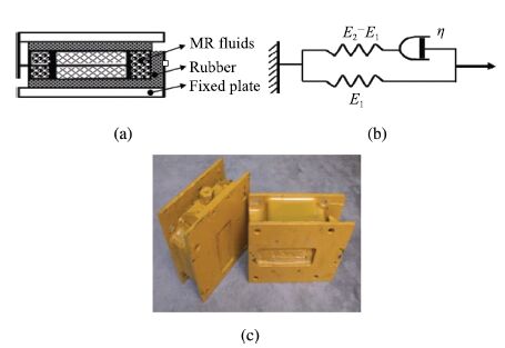
In Fig. 2, the shock absorber is composed of an MR damper and a
rubber damper,which possesses the advantages of the rubber and the
MR damper. The damping force can be adjusted rapidly with little
control energy requirement. In view of the structural
characteristics of the coupled shock absorber,a typical standard
linear solid model is presented,also called the Zener
model[10],as shown in Fig. 2(b). The fractional order Zener
model can be obtained by replacing the traditional Newton dashpot
with the Abel dashpot. The constitutive relation can be written
as[10]:
\begin{equation}
\sigma+\tau^{\alpha}D^{\alpha}\sigma(t)=E_2\tau^{\alpha}D^{\alpha}\varepsilon(t)
+E_1\varepsilon(t),\ \ 0\leq \alpha<1,
\end{equation}
(8)
$$E' = {{{E_2}{{(\omega \tau )}^{2\alpha }} + {{(\omega \tau )}^\alpha }({E_1} + {E_2})\cos \left( {\alpha {\pi \over 2}} \right) + {E_1}} \over {{{\left[ {1 + {{(\omega \tau )}^\alpha }\cos \left( {\alpha {\pi \over 2}} \right)} \right]}^2} + {{\left[ {{{(\omega \tau )}^\alpha }\sin \left( {\alpha {\pi \over 2}} \right)} \right]}^2}}},$$
(9)
$$E'' = {{({E_2} - {E_1}){{(\omega \tau )}^\alpha }\sin \left( {\alpha {\pi \over 2}} \right)} \over {{{\left[ {1 + {{(\omega \tau )}^\alpha }\cos \left( {\alpha {\pi \over 2}} \right)} \right]}^2} + {{\left[ {{{(\omega \tau )}^\alpha }\sin \left( {\alpha {\pi \over 2}} \right)} \right]}^2}}},$$
(10)
|
Download:
|
| Fig. 2 The principle of the damper and the simplified model: (a) The schematic diagram of the shock absorber; (b) Simplified model; (c) The shock absorber. | |
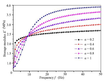
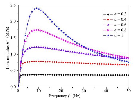
Substituting the structure parameters obtained from the coupled shock absorber into the (9) and (10),the storage modulus ($E'$) and loss modulus ($E''$) can be calculated,shown in Figs.3 and 4. The storage modulus $E'$ increases as a function of the system frequency,while the loss modulus $E''$ is nonlinear. Using verified parameters and changing the order of the Abel dashpot from 0.2 to 1, $E'$ and $E''$ exhibit different characteristics. When the frequency is less than 10 Hz,$E'$ decreases with the increase of the order $\alpha$. When the frequency is larger than 10 Hz,the law is opposite,showing that the smaller $\alpha$ produces larger elastic properties of the shock absorber. When $0<\alpha<1$,the $E''$ increases with the increase of the order $\alpha$,showing an increase in the viscous behavior. When $\alpha=1$,the $E''$ has a fast drop when the frequency is larger than 10 Hz,when the frequency increases beyond a certain value,the loss modulus is smaller than a small $\alpha$,as the Fig. 4 showing,the loss modulus in $\alpha=1$ is smaller than $\alpha=0.8$ when the frequency is larger than 32 Hz.
|
Download:
|
| Fig. 3 The storage modulus of Zener model $E'$. | |
|
Download:
|
| Fig. 4 The loss modulus of Zener model $E''$. | |
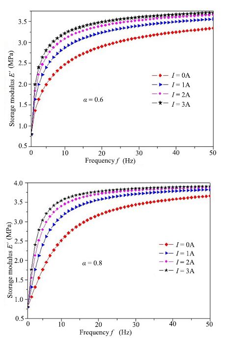
When the applied magnetic field is manipulated according to the damping part of the coupled MR damper,the viscoelastic properties of the entire shock absorber can be changed dramatically. The magnetic field can be manipulated by changing the current,$I$,of the system. In Fig. 5, the storage modulus is plotted as a function of frequency for two different values of $\alpha$. In Fig. 5(a), as $I$ is increased,the storage modulus asymptote increases. Also as $I$ is increased,the storage modulus approaches the asymptote more rapidly. In Fig. 5(b) the asymptotic value of each current is larger than the corresponding current in Fig. 5(a). Similar to Fig. 6(a), the storage modulus gradually approaches the asymptote as frequency is increased. As $I$ is increased,the storage modulus approaches the asymptote much more rapidly.
|
Download:
|
| Fig. 5 The storage modulus $E'$ of the Zener model with different currents. | |
|
Download:
|
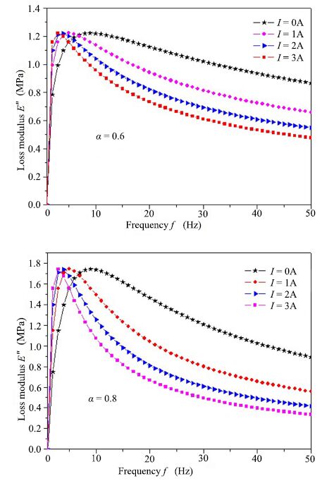
| Fig. 6 The loss modulus $E''$ of the Zener model with different currents. | |
In Fig. 6, the loss modulus is plotted as a function of frequency. In Fig. 6(a), for $I=0$,the loss modulus reaches a maximum for $f=8$. As frequency is increased,the loss modulus gradually decreases. For $I>0$,the modulus rapidly increases and reaches a maximum value for $f=4$. The maximums for all values of $I$ are all very similar in magnitude. However,as frequency is increased, larger currents possess a smaller loss modulus. In Fig. 6(b), for $I=0$,the maximum in loss modulus occurs at $f=8$. The loss modulus then gradually decreases. For $I>0$,the maximum occurs for $f$ $=$ $4$. Furthermore,the decrease in loss modulus is much more rapid than what we observed in Fig. 6(a) for $\alpha=0.6$. In addition, the maximum for all values of $I$ is larger than the maximums observed in Fig. 6(a). The viscous characteristics of the coupled MR damper are reflected in the low working frequency. At large frequency the viscous performance of the damper is decreased,which is directly related to the working magnetic field.
Ⅲ. Experimental PlatformFrom the above analysis,it can be seen that the fractional order model can accurately describe the viscoelasticity of the shock absorber. In order to further the study and analyze the dynamic performance of the damper,equivalent viscous damping is introduced[11]. The equivalent viscous damping is used to replace the complex damping machine.
A. Experiment Platform and Model Analysis
From (8),the resistance,$f(t)$,is provided,and the direction is
opposite to the speed of the mass,$m$. The force applied to the
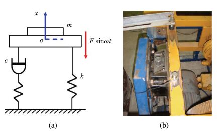
system is $F\sin\omega t$,as shown in Fig. 7(a), the two-order
mode for a single degree of freedom dynamic system is defined as:
\begin{equation}
m\ddot{x}(t)+c\dot{x}(t)+kx(t)=F\sin\omega t,
\end{equation}
(11)
\begin{equation}
\ddot{x}(t)+2\mu\omega_n^2\dot{x}(t)+\omega_n^2x(t)=\frac{F\sin\omega
t}{m},
\end{equation}
(12)
| \begin{equation} D^2x(t)+2\mu\omega_nD^{\beta}x(t)+\omega_n^2x(t)=P(t),\ \ 0<\beta\leq 1. \end{equation} | (13) |
|
Download:
|
| Fig. 7 The simplified model and the real experimental platform: (a) The simplified model of the experimental platform; (b) The real experimental platform. | |
In order to simplify (13),here $A_1=\mu\omega_n$,$A_2=w_n^2$,so
(13) can be written as follows:
\begin{equation}
D^2x(t)+A_1D^{\beta}x(t)+A_2x(t)=F(t).
\end{equation}
(14)
\begin{equation}
s^2X(s)+A_1s^{\beta}X(s)+A_2X(s)=F(s).
\end{equation}
(15)
| \begin{equation} G(s)=\frac{1}{s^2+\mu^{\beta}\omega_n^{\beta}s^{\beta}+\omega_n^2},\ \ 0<\beta<2. \end{equation} | (16) |
For the differential equation (11),the Grünwald-Letnikov (G-L) definition is used to solve the differential equation. The Grünwald-Letnikov method is the direct numerical method for solving fractional calculus.
The G-L definition of fractional calculus is as follows:
\begin{align}\nonumber
{}_aD_t^{\beta_i}x(t)=&\ \frac{1}{h^{\beta_i}}\sum_{j=0}^{\frac{t-a}{h}}w_j^{(\beta_i)}x_{t-jh}\\
=&\ \frac{1}{h^{\beta_i}}\left[x_t+\sum_{j=1}^{\frac{t-a}{h}}
w_j^{(\beta_i)}x_{t-jh}\right].
\end{align}
(17)
\begin{equation}
w_0^{\beta_i}=1,\ w_j^{(\beta_i)}=\left(1-\frac{\beta_i+1}{j}
\right)w_{j-1}^{(\beta_i)},\ \ j=1,2,\ldots.
\end{equation}
(18)
\begin{equation}
x_t=\frac{1}{\displaystyle\sum_{i=0}^n\frac{a_i}{h^{\beta_i}}}
\left[P(t)-\sum_{i=0}^n\frac{a_i}{h^{\beta_i}}\sum_{j=1}^{\frac{t-a}{h}}w_j^{(\beta_i)}x_{t-jh}
\right],
\end{equation}
(19)
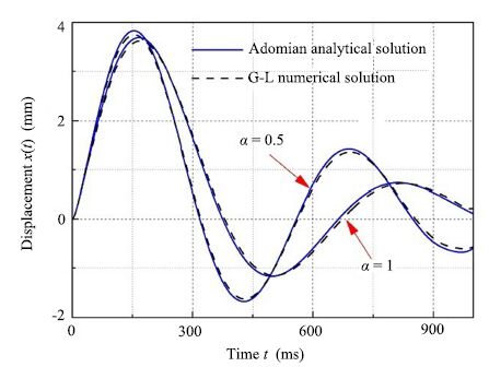
The numerical solution and the analytical solution for the trinomial model (i.e.,$\alpha_2=2$,$\alpha_1=\alpha$,$\alpha_0=0$) excited by unit step function are shown in Fig. 8. The solutions are calculated based on (15) and by the method of Adomian decomposition, respectively. In Fig. 8, the displacement is plotted as a function of time. From Fig. 8, both the numerical and analytical solutions exhibit similar displacement for all values of time considered. Therefore,the numerical solution of G-L can be applied to engineering analysis. In this paper,the fractional order model and the integer order model are analyzed using the numerical solution.
|
Download:
|
| Fig. 8 Adomian decomposition method solution vs G-L definition numerical solution. | |
B. Measurement and Control Device
The measurement and control system of MR damper is shown in Fig. 7. In the MR damper,the sensor collects the signals of vibration, displacement and acceleration. LabVIEW is used to process,analyze, and display the collected data. Then,based on the specific vibration control requirements and other related parameters (system structure,magnetorheological material characteristics,etc.),the required control current is calculated using the GBIP mode in LabVIEW. Through LabVIEW,the vibrational damping force can be controlled. The changes to the vibrational parameters of the experimental platform can be observed,and the output current can be adjusted to achieve a more desirable vibrational damping effect. The response of the shock absorber is of the order of several tens of milliseconds. A high signal sampling rate is required in order to meet the required vibrational reduction.
The system consists of temperature,acceleration,and displacement sensors,as well as a data acquisition card of virtual instrument system,data acquisition terminal,software system using LabVIEW7.0 version,programmable current source,etc.
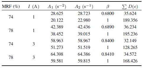
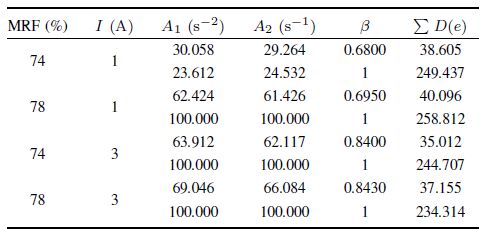
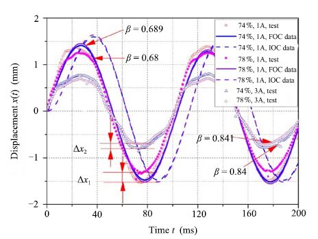
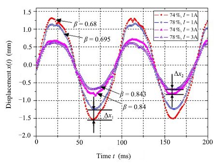
Ⅳ. Experiment AnalysisThe dynamic characteristics in the MR fluids are considered with changing mass percent of carbonyl iron. In Figs.9 and 10,the mass percentages of carbonyl considered are 74 % and 78 %. The eccentricity is large for vibration frequencies of 10 Hz and 11 Hz. The dynamic parameters of the system model are described in Tables Ⅰ and Ⅱ.
|
|
Table Ⅰ $f=10$ Hz,THE PARAMETERS $A_1$,$A_2$,$\beta$,$D(e)$ OF THE MODEL IN DIFFERENT WORKING FLUIDS |
|
|
Table Ⅱ $f=11$ Hz,THE PARAMETERS $A_1$,$A_2$,$\beta$,$D(e)$ OF THE MODEL UNDER DIFFERENT WORKING FLUIDS |
1) The order $\beta$ of fractional order model is related to the vibration damping performance of MR fluids. With the same control current and the nonmagnetic saturation situation,the damping capacity and the model order $\beta$ increase with the increase of the mass fraction of the carbonyl iron powder. As shown in Fig. 9, at $f=10$ Hz,$I=1$ A,the fractional order $\beta$ increases from 0.68 to 0.689 as mass fraction $M$ increased from 74 % to 78 % accordingly. Similar situation can be seen from Fig. 10, at $f=11$ Hz,$I=1$ A,the fractional order $\beta$ increases from 0.68 to 0.695 as mass fraction $M$ adjusted from 74 % to 78 %. From the results we can find that the order number is changed with the different working fluids.
|
Download:
|
| Fig. 9 $f=10$ Hz,the displacements and the fractional order in different working fluids. | |
|
Download:
|
| Fig. 10 $f=11$ Hz,the vibration displacements and the fractional order in different working fluids. | |
2) The viscoelastic characteristics of the system with higher iron content is stronger: such as,$f=10$ Hz,$I=1$ A,when $M=74$ %, 78 % respectively,the viscosity coefficients of $A_1$ are 28.625, 42.389,which shows a significant increase; viscoelastic ratio $\xi$ is respectively 0.9965 and 0.9988,which is also increased weakly, so can also be viewed unchanged.
3) $\Delta x_1$ and $\Delta x_2$ represent the variation displacement of the two working fluids in 1 A,3 A respectively, it can be seen that $\Delta x_1>\Delta x_2$,and under the working current of 3 A,the changes of MR fluids damping characteristics are reducing.
4) The displacement of the theoretical fractional model and the integer order model are given in Figs.9 and 10. It can be seen that the fitting curve of fractional order model is more close to the sampled displacement curve than that of the integer order model, and the results are in agreement with the computed results of Tables Ⅰ and Ⅱ. Based on the same sampled signal,the residual sum of squares $\sum D(e)$ obtained by fitting the fractional order models is less than that of the integer order models obtained by fitting the integer model,indicating that the fractional order system model is more accurate than the integer order system model.
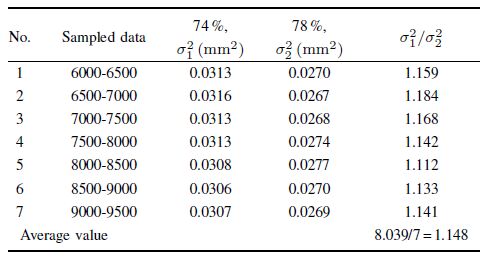
The effect of working fluids on the vibrational energy of the system is analyzed quantitatively by using the variance analysis. As shown in Table Ⅲ,taking $I=1$ A in Fig. 9 for example,$\sigma_1^2$ is the variance at $M=74$ %,and $\sigma_2^2$ is variance at $M=78$ %,$\sigma_1^2/\sigma_2^2$ denotes the energy coefficient, we can find that the replacement of the working fluids has great influence on the dynamic energy coefficient,whose average value is 1.148,indicating that different MR liquids of the system have certain influence on the system.
|
|
Table Ⅲ $I=1$ A,THE VARIANCE OF THE SAMPLED DATA SEGMENTS WITH DIFFERENT CURRENTS |
The above analysis shows the mechanical properties of the coupled MR damper using viscous and elastic characteristics,presenting the properties of an elastic solid and a viscous fluid,and through the experiment,we have shown that:
1) the constitutive equation with fractional derivative method is derived from a strict formula,which has definite physical meaning;
2) the viscoelastic constitutive equation with the fractional derivative can be used to describe the mechanical vibration performance of the coupled MR damper with great accuracy than the integer order model;
3) the dynamic characteristics of the system are related to the order number of the fractional order model: under the same operating frequency,with the increase of the control current,the order of the fractional model is increased,and the viscoelastic properties of the shock absorber are enhanced.
| [1] | Stanway R, Sproston J L, Stevens N G. Non-linear modelling of an electro-rheological vibration damper. Journal of Electrostatics, 1987, 20(2): 167-184 |
| [2] | Spencer B F Jr, Dyke S J, Sain M K, Carlson J D. Phenomenological model for magnetorheological damper. Journal of Engineering Mechanics, 1997, 123(3): 230-238 |
| [3] | Zhou Qiang, Qu Wei-Lian. Two mechanic models for magnetorheological damper and corresponding test verification. Earthquake Engineering and Engineering Vibration, 2002, 22(4): 144-150 (in Chinese) |
| [4] | Gamota D R, Filisko F E. Dynamic mechanical studies of electrorheological materials: moderate frequencies. Journal of Rheology, 1991, 35(3): 399-425 |
| [5] | Slonimsky G L. Laws of mechanical relaxation processes in polymers. Journal of Polymer Science Part C: Polymer Symposia , 1967, 16(3): 1667-1672 |
| [6] | Friedrich C. Relaxation and retardation functions of the maxwell model with fractional derivatives. Rheologica Acta, 1991, 30(2): 151-158 |
| [7] | Bagley R L, Torvik P J. On the fractional calculus model of viscoelastic behavior. Journal of Rheology, 1986, 30(1): 133-155 |
| [8] | Paggi M, Sapora A. An accurate thermoviscoelastic rheological model for ethylene vinyl acetate based on fractional calculus. International Journal of Photoenergy, 2015, 2015: Article ID 252740 |
| [9] | Jóźwiak B, Orczykowska M, Dziubiński M. Fractional generalizations of maxwell and kelvin-voigt models for biopolymer characterization. PLoS One, 2015, 10(11): e0143090 |
| [10] | Alcoutlabi M, Martinez-Vega J J. Application of fractional calculus to viscoelastic behaviour modelling and to the physical ageing phenomenon in glassy amorphous polymers. Polymer, 1998, 39(25): 6269-6277 |
| [11] | Li Zhuo, Xu Bing-Ye. Equivalent viscous damping system for viscoelastic fractional derivative model. Journal of Tsinghua University (Science and Technology), 2000, 40(11): 27-29 (in Chinese) |
| [12] | Wang Zhen-Bin, Cao Guang-Yi, Zhu Xin-Jian. Application of fractional calculus in system modeling. Journal of Shanghai Jiaotong University, 2004, 38(5): 802-805 (in Chinese) |
| [13] | Wang Zhen-Bin, Cao Guang-Yi. Two system modeling methods using fractional calculus. Journal of System Simulation, 2004, 16(4): 810-812 (in Chinese) |
| [14] | Xue D Y, Chen Y Q. Solving Applied Mathematical Problems with Matlab. Boca Raton: CRC Press, 2008. |
 2016, Vol.3


