2. Department of Control Science and Engineering, Jilin University (Campus Nanling), Changchun 130025, China;
3. Jilin University, Changchun 130012, China
GENERALLY, the electrochemical reactions inside lithium-ion battery are complicated in the running electric vehicle (EV), which is a highly nonlinear dynamic system. State of charge (SOC)[1] is defined as the percentage of the amount of left energy to the rated capacity of a battery, which cannot be measured directly, it only can be estimated by measured variables such as current and terminal voltage. The accurate estimation of SOC is the key problem in the field of power battery.
The methods of SOC estimation are categorized into direct experiment measurement methods and estimation methods based on battery models. Coulomb counting method and current integration method are the most popular experiment measurement methods, which are simple to obtain SOC. However, these methods result in high errors caused by the accumulation of errors in numerical integration in current measurement. State observer[2, 3], Kalman filter (KF)[4, 5] and particle filter (PF)[6, 7] are used to estimate SOC based on the model of Lithium-ion battery. The SOC estimation error of each method is summarized in [8], which shows that the existing integer order battery SOC estimation methods mainly have estimation error larger than 1%, which may be because the models which are obtained through the external characteristics of the power battery cannot show the precise internal characteristics. The dynamics of the battery is described by a set of integer order calculus equations. But complex electrochemical reactions are described by the fractional order function.
The fractional order calculus (FOC) is a natural extension of the classical integral order calculus. References [9$-$11] have shown that most phenomena, such as damping, friction, mechanical vibration, dynamic backlash, sound diffusion, etc., have fractional order properties. Thus, FOC is widely used in modeling, kinetics estimation, etc. FOC is also used to develop the electrochemical models of the super capacitors and so on.
When it comes to FOC battery modeling and SOC estimation, [12] uses FOC model obtained by system identification to estimate crankability of battery, [13] proposes lead acid battery state of charge estimation with FOC, and [14] deals with a fractional order state space model for the lithium-ion battery and its time domain system identification method. The existing FOC modeling for battery meets the same problem, the estimation accuracy in not high enough for battery management system.
The electrochemical impedance spectroscopy (EIS) method is one of the most accurate methods to model the electrochemical Li-ion batteries. There are many studies which have tried to utilize the impedance spectra directly to estimate SOC, but EIS method is too complicated to be used directly. EIS method is mainly used with equivalent circuit model at present[15, 16].
The remainder of the paper is organized as follows. Section II discusses the battery fractional-order modeling based on impedance spectra; Section III discusses how to obtain characteristic curve between open circuit voltage (OCV) and SOC, states order identification with frequency method and parameters identification according to the output error identification algorithm; Section IV presents fractional order Kalman filter for SOC estimation; Section V draws conclusions from the preceding work and offers suggestion for further study.
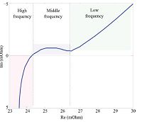
Ⅱ. FRACTIONAL MODELLING OF BATTERYThe impedance spectra curve of the Lithium-ion battery can be got through Electrochemical workstation and is shown in Fig. 1. As shown in the figure, the impedance spectra can be divided into three sections: the high frequency section, the mid frequency section and the low frequency section.
|
Download:
|
| Fig. 1 Impedance spectra of a Li-ion battery. | |
In the high frequency section, the impedance spectra curve intersects with the real axis and the intersection point could be represented by an Ohmic resistance.
In the low frequency section, the impedance spectra curve is a straight line with a constant slope, and has the same impedance spectroscopy characteristic with constant phase element (CPE) which is usually referred to as a Warburg element.
The middle frequency section forms a depressed semicircle, which is a well-known phenomenon in electrochemistry. Such a depressed semicircle could be modeled by paralleling a Warburg element or CPE with a resistance, which is referred to as a ZARC element (it yields an arc in the $Z$ plane)[17].
From the analysis above, the equivalent circuit model can be described as Fig. 2. $V_{oc}$ denotes open circuit voltage (OCV), and $V_{o}$ denotes battery terminal voltage which can be directly measured; $R_{1}\in{\bf R}$ denotes the value of Ohmic resistance, $I$ denotes the current, and $V_{1}$ denotes the voltage of $R_{1}$; $C_{2}$ $\in$ ${\bf R}$ is the coefficient of CPE in ZARC element, $R_{2}\in{\bf R}$ denotes the value of Ohmic resistance in ZARC element, and $V_{2}$ denotes the terminal voltage of ZARC element; $W\in{\bf R}$ is the coefficient of Warburg element, and $V_{3}$ denotes the voltage of Warburg element.

|
Download:
|
| Fig. 2 Solution representation in the EDA-IG. | |
From the above description, the battery can be described by a fractional model. To simplify the FOC equation, we define the denotation as follows:
| ${{\Delta }^{r}}=\left\{ \begin{array}{*{35}{l}} \frac{{{\text{d}}^{r}}}{\text{d}{{t}^{r}}}, & r>0, \\ [1mm]1, & r=0, \\ [1mm]\int{{{(\text{d}\tau )}^{r}}}, & r<0. \\ \end{array} \right.$ |
The mathematical model in high frequency can be described as (1).
| \begin{align} \label{eq:1} V_{1}=R_{1}I, \end{align} | (1) |
where $R_{1}\in{\bf R}$ denotes the value of Ohmic resistance, $I$ denotes the current, and $V_{1}$ denotes the voltage of $R_{1}$.
The mathematical model in middle frequency can be described as (2).
| \begin{align} \label{eq:2} \Delta^{\beta}V_{2}=-{{1}\over {R_{2}C_{2}}}V_{2}-{{1}\over {C_{2}}}I, \end{align} | (2) |
The mathematical model of Warburg element in low frequency can be described as (3).
| \begin{align} \label{eq:3} \Delta^{\alpha}V_{3}=-{{1}\over{W}}I, \end{align} | (3) |
where $W\in{\bf R}$ is the coefficient, $\Delta^{\alpha}$ denotes $\alpha$ order of the fractional element, $\alpha\in{\bf R}$, $-1<\alpha<1$ is the fractional order of Warburg element, $V_{3}$ denotes the voltage of Warburg element, and $I$ denotes the current across the Warburg element.
For the determined relationship of OCV and SOC, SOC can be regarded as a system state, which can be presented as follows:
| \begin{align} \label{eq:4} \Delta^{1}S_{oc}=-{{1}\over{Q_{n}}}I, \end{align} | (4) |
The relationship between SOC and OCV is nonlinear and it is not easy to draw a mathematical interpretation for it. It is easy to find that when SOC is between 20% and 80% the relationship is considered to be linear and can be written as follows:
| \begin{align} \label{eq:5} V_{oc}=k\cdot{S_{oc}}+d, \end{align} | (5) |
where $k$ and $d$ are the coefficients which can be calculated from the curve fitting.
Set the system state vector as $x=\left[\begin{array}{ccc}V_{2}&V_{3}&S_{oc}\\\end{array}\right]^{\rm T}$, the system input as $u=I$, and the system output as $y=V_{o}-d$. The continuous fractional state space function can be written as (6).
| \begin{align} \label{eq:6} \begin{cases} \Delta^{N}x=Ax+Bu, \\ y=Cx+Du, \end{cases} \end{align} | (6) |
where $A=\left[\begin{array}{ccc}-{{1}\over {R_{2}C_{2}}}&0&0\\0&0&0\\0&0&0\\\end{array}\right]$, $B=\left[\begin{array}{c}-{{1}\over {C_{2}}}\\[1mm]-{{1}\over {W}}\\[1mm]-{{1}\over {Q_{n}}}\\\end{array}\right]$, $C=$ $\left[\begin{array}{ccc}1&1&k\\\end{array}\right]$, $D=-R_{1}$, $N=\left[\begin{array}{c}\beta\\\alpha\\1\\\end{array}\right]$.
According to the stochastic theory, the discrete state space function is obtained as follows:
| \begin{align} \label{eq:7} \begin{cases} \Delta^{N}x_{k+1}=Ax_{k}+Bu_{k}, \\ y_{k}=Cx_{k}+Du_{k}, \end{cases} \end{align} | (7) |
where $x_{k}\in{{\bf R}^{3}}$ denotes the system state vector, $y_{k}\in{\bf R}$ denotes the system output, and $u_{k}\in{\bf R}$ denotes the system input, all at the time instant $k$.
The fractional order Grünwald-Letnikov definition is given as
| \begin{align} \label{eq:8} \Delta^{N}{x_{k}}={{1}\over {T_{s}^{N}}}\sum_{j=0}^k(-1)^{j}\left(\begin{array}{c} N\\j\end{array}\right)x_{k-j}, \end{align} | (8) |
where $T_{s}$ is the sample interval, and $k$ is the number of samples for which the derivative is calculated,
| \begin{align*}\left(\begin{array}{c}N\\j\end{array}\right)=\begin{cases} 1, &j=0, \\[1mm] \frac{N(N-1)\cdots(N-j+1)}{j!}, &j>0. \end{cases}\end{align*} |
Equation(9) can be derived from(8).
| \begin{align} \label{eq:9} x_{k+1}=&\ T_{s}^{N}\Delta^{N}{x_{k+1}}-\left(\begin{array}{c}N\\1\end{array}\right)x_{k}\nonumber\\ & +\sum_{j=2}^{k+1}(-1)^{j}\left(\begin{array}{c} N\\j\end{array}\right)x_{k-j+1}. \end{align} | (9) |
The discrete state space function of the battery can be written as (10).
| \begin{align} \label{eq:10} \begin{cases} x_{k+1}=T_{s}^{N}(A+NE)x_{k}+T_{s}^{N}Bu_{k}-\sum\limits_{j=2}^{k+1}\gamma_{j}x_{k-j+1}, \\ y_{k}=Cx_{k}+Du_{k}, \end{cases} \end{align} | (10) |
where $\gamma_{j}={\rm diag}\left\{\left(\begin{array}{c}\beta\\j\end{array}\right)\left(\begin{array}{c}\alpha\\j\end{array}\right)\left(\begin{array}{c}1\\j\end{array}\right)\right\}$.
Let $A_{d}=T_{s}^{N}(A+NE)$, $B_{d}=T_{s}^{N}B$, $C_{d}=C$, $D_{d}=D$, and $E$ be unit matrix. Considering the process noise and output noise, the discrete state space function of the system can be written as
| \begin{align} \label{eq:11} \begin{cases} x_{k+1}=A_{d}x_{k}+B_{d}u_{k}+w_{k}-\sum\limits_{j=2}^{k+1}\gamma_{j}x_{k-j+1}, \\ y_{k}=C_{d}x_{k}+D_{d}u_{k}+v_{k}, \end{cases} \end{align} | (11) |
where $w_{k}\in{{\bf R}^{3}}$ is process noise, representing the modeling uncertainty and unknown input, $v_{k}\in{\bf R}$ is output noise, on behalf of the measurement disturbance, $w_{k}$ and $v_{k}$ are assumed to be independent, zero mean Gaussian noise processes with the covariance matrices ${\rm E}[w_{k}w_{j}^{\rm T}]=Q_{k}\delta_{kj}$, ${\rm E}[v_{k}v_{j}^{\rm T}]=R_{k}\delta_{kj}$, and $\delta_{kj}$ is Kronecker function.
Ⅲ. PARAMETER IDENTIFICATIONParameter identification of battery model can be divided into two sections, curve fitting of relationship between OCV and SOC and parameter identification in battery model. We will describe the two parts separately as following.
A. Curve Fitting Between OCV and SOCOCV is obtained by fitting average value of charging and discharging terminal voltages which are measured by applying constant pulse current for each time 10% SOC to battery in both of charging and discharging modes.
Through the above test, the unknown parameters $k$ and $d$ in(5) can be obtained by curve fitting.
The specific test procedure is as follows:
1) Discharge the battery till it reaches the minimum discharging voltage (2 V in our case) at room temperature, and keep it idle for 12 hours.
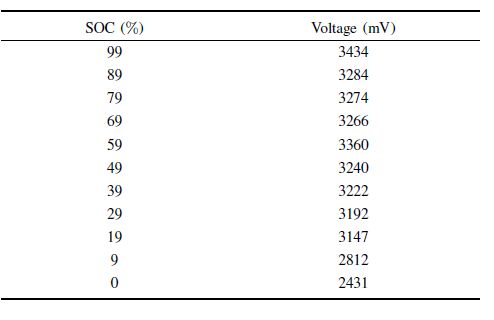
2) Charge the battery with a constant current of 0.2 C (0.5 A) till terminal voltage reaches 3.7 V. During the procedure, idle the battery for 2 minutes after each 10% SOC charging. Record every minimum voltage, as shown in Table I.
|
|
Table Ⅰ MINIMUM POINTS OF EVERY SOC WHILE CHARGING |
3) Idle the battery for 12 hours.
4) Discharge the battery with a constant current of 0.2 C (0.5 A) till terminal voltage reaches 2 V. During the procedure, idle the battery for 2 minutes after each 10% SOC discharging. Record every maximum voltage, as shown in Table II.
|
|
Table Ⅱ MAXIMUM POINTS OF EVERY SOC WHILE DISCHARGING |
5) Fit minimum points and maximum points that we collected in prior experiments respectively and average the two curves, which are shown in Fig. 3.

|
Download:
|
| Fig. 3 SOCV measurement during charging and discharging. | |
Fitting the OCV-SOC relationship from 20% SOC to 80% SOC as shown in Fig. 4, we can get the values $k=0.002086$ and $d=3.166$.

|
Download:
|
| Fig. 4 OCV-SOC curves between 20% and 80% SOC. | |
Identify unknown parameters in (6) with time domain and frequency domain method separately.
1)Identify the order of states using frequency fitting method in frequency domain: This impedance spectra curve of the Warburg element has the slope of ${\alpha\pi}/{2}$. The slope of the low-frequency part of the impedance spectra is nearly ${\pi}/{4}$, so parameter $\alpha$ is equal to $0.5$.
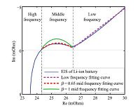
The impedance spectra curve of the loop consisting of a CPE and a resistance is shaped like a semicircle. The regression rate of the semicircle will be changed with $\beta$. The bigger $\beta$ is, the bigger the curve radian is. When $\beta=0.65$, the measured impedance spectra will be matched well, shown in Fig. 5.
|
Download:
|
| Fig. 5 System state order fitting curve. | |
Fig. 5 shows that the impedance spectra curve obtained by the order of state identification can match the measured impedance spectra well, which means that the fractional-order model can express the characteristic of Lithium-ion battery well.
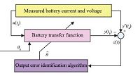
2)Unknown parameter identification: Unknown parameters are identified via output error identification algorithm in time domain[18, 19]. The output error approach is diagrammed in Fig. 6.
|
Download:
|
| Fig. 6 Parameter identification of battery by output error approach. | |
The transfer function of fractional order equivalent circuit model shown in Fig. 1 can be written as
| \begin{align} \label{eq:12} H(s)&={{V(s)}\over{I(s)}}={{1}\over{Ws^{\alpha}}}\cdot{R_{1}} \cdot{{R_{2}(\frac{1}{C_{2}s^{\beta}})}\over{R_{2}+(\frac{1}{C_{2}s^{\beta}})}}\notag\\ &={{R_{1}R_{2}}\over{Ws^{\alpha}(1+C_{2}R_{2}s^{\beta}})}, \end{align} | (12) |
where $V=V_{o}-V_{oc}$.
Equation(12) can be written as(13).
| \begin{align} \label{eq:13} V(s)Ws^{\alpha}(1+C_{2}R_{2}s^{\beta})=I(s)R_{1}R_{2}. \end{align} | (13) |
Applying of inverse Laplace transform algorithm, we have
| \begin{align} \label{eq:14} W{{{\rm d}^{\alpha}}\over{{\rm d}t}}V(t)+C_{2}R_{2}W{{{\rm d}^{\alpha+\beta}}\over{{\rm d}t}}V(t)=R_{1}R_{2}I(t). \end{align} | (14) |
Let $a=R_{1}R_{2}$, $b=W$, $c=C_{2}R_{2}W$, $\theta=\left[\begin{array}{c}a\\b\\c\\\end{array}\right]$, $p={\dfrac{\rm d}{\rm dt}}$. Equation(14) is written as
| \begin{align} \label{eq:15} G(p)={{V(t)}\over{I(t)}}={{a}\over{bp^{\alpha}+cp^{\alpha+\beta}}}={{B(\theta)}\over{A(p, \theta)}}. \end{align} | (15) |
The noise-free output $y(t_{k})$ is supposed to be corrupted by an additive white measurement noise $v(t_{k})$ which is normally distributed with a zero mean and $R$ variance, considered at discrete instants. The complete equation can be written in the form
| \begin{align} \label{eq:16} \begin{cases} y(t_{k})=G(p)\cdot{u(t_{k})}, \\ y^{*}(t_{k})=y(t_{k})+v(t_{k}), \end{cases} \end{align} | (16) |
where $y^{*}(t_{k})$ is the measured output of the system.
Assume that an error function $\varepsilon(t)$ is given by the output error, i.e.,
| \begin{align} \label{eq:17} \varepsilon(t) &=y^{*}(t_{k}, \theta)-\frac{B(\theta)}{A(p, \theta)}u(t)\notag\\ &=A(p, \theta)\left(\frac{y^{*}(t_{k}, \theta)}{A(p, \theta)}\right)-B(\theta)\left(\frac{u(t)}{A(p, \theta)}\right)\notag\\ &=A(p, \theta)y_{f}^{*}(t)-B(\theta)u_{f}(t), \end{align} | (17) |
where $y_{f}^{*}(t)={y^{*}(t, \theta)}/{A(p, \theta)}$ and $u_{f}(t)={u(t)}/{A(p, \theta)}$. Hence, a linear low-pass filter is applied to the measured input part and output part separately instead of a direct differentiation of the input variable and output variable. As shown in (17), the filter converts the output error into an equation error[20].
Let $F^{n}(p)={1}/{A(p, \theta^{n})}$, $n=1, 2, \ldots$ stands for the iteration number. In practical cases, $A(p, \theta)$ being unknown, an estimation $F^{n}(p)={1}/{\hat{A}(p, \hat{\theta}^{n})}$ is computed iteratively.
The noise-free output variable is obtained through an auxiliary model, i.e.,
| \begin{align} \label{eq:18} y^{n}(t)=\frac{\hat{B}(\hat{\theta}^{n})}{\hat{A}(p, \hat{\theta}^{n})}u(t). \end{align} | (18) |
The filtered input, output, and measured output are computed respectively with
| \begin{align*} &u_{f}(t)=F^{n}(p)u(t), \\ &p^{\alpha}y_{f}(t)=p^{\alpha}F^{n}(p)y(t), \\ &p^{\alpha}y^{*}_{f}(t)=p^{\alpha}F^{n}(p)y^{*}(t). \end{align*} |
And they are gathered in the regression vectors as
| \begin{align*} &\varphi_{f}(k)=\left[\begin{array}{ccc}u_{f}(k)&-p^{\alpha}y^{*}_{f}(k)&-p^{\alpha+\beta}y^{*}_{f}(k)\end{array}\right]^{\rm T}, \\ &\varphi^{n}_{f}(k)=\left[\begin{array}{ccc}u_{f}(k)&-p^{\alpha}y_{f}(k)&-p^{\alpha+\beta}y_{f}(k)\end{array}\right]^{\rm T}.\end{align*} |
Thus, we have
| \begin{align}\label{eq:19} &\Phi^{n}_{f}=\left[\begin{array}{ccc}\varphi^{n}_{f}(0)&...&\varphi^{n}_{f}(T_{\rm final})\end{array}\right], \notag\\ &\Phi_{f}=\left[\begin{array}{ccc}\varphi_{f}(0)&...&\varphi_{f}(T_{\rm final})\end{array}\right], \notag\\ &Y_{f}^{\ast}=\left[\begin{array}{ccc}y_{f}^{\ast}(0)&...&y_{f}^{\ast}(T_{\rm final})\end{array}\right]. \end{align} | (19) |
The optimization problem of the parameter identification can be stated as
| \begin{align} \label{eq:20} \hat{\theta}_{k}=\arg\min_{\theta} \left \| [\Phi^{n}_{f}\Phi_{f}^{\rm T}]\theta-[\Phi_{f}^{n}Y^{*}_{f}] \right \|^{2}. \end{align} | (20) |
The solution is given by
| \begin{align} \label{eq:21} \hat{\theta}_{k}=(\Phi^{n}_{f}\Phi_{f}^{\rm T})^{-1}\Phi_{f}^{n}Y^{*}_{f}, \end{align} | (21) |
and the algorithm is iterated until convergence, when $\max{| \frac{\hat{\theta}_{k}-\hat{\theta}_{k-1}}{\hat{\theta}_k} |}$ $<$ $\varepsilon$ , where $\varepsilon$ is chosen by the accuracy of modeling.
Specific identification process can be described as:
1) $k=0$, initialize the parameters with $\theta_{0}=\begin{bmatrix}0&0&0\end{bmatrix}^{\rm T}$.
2) $ k=1, 2, 3, \ldots$, calculate noise-free output $y(k)$ according to $\theta_{k-1}$ and(16).
3) Filter the current, the terminal voltage, and the noise-free terminal voltage based on(18).
4) Determine variables based on(19).
5) Update the identified parameters $\hat{\theta}_{k}$ by(21).
6) Calculate the relative error of $ | \frac{\hat{\theta}_{k}-\hat{\theta}_{k-1}}{\hat{\theta}_{k}} |$ from 2) to 5) until the error is less than $0.05$.
After the identification process, the value of every element can be gotten as $R_{2}=\frac{a}{R_1}$, $ W=b $, $C_2=\frac{c}{R_{2}W}$ in (6), $Q_{n}$ $=$ $C_{n}\times 3600$ where $C_{n}$ is the nominal capacity, i.e., $R_2=$ $2.1 {\rm m}\Omega$, $W=26.5$, $ C_2=11 {\rm mF}$.
The intersection of impedance spectra with real axis in high frequency shows the value of resistance. From the impedance spectra curve we can get $R_1=24.3 {\rm m}\Omega$.
Bring the above parameters into(6), the discrete fractional model can be written as
| \begin{align}\label{eq:22} \begin{cases} x_{k+1} =A_{d}x_{k}+B_{d}u_{k}+w_{k}-\sum\limits_{j=2}^{k+1}\gamma_{j}x_{k-j+1}, \\ y_{k} =C_{d}x_{k}+D_{d}u_{k}+v_{k}, \end{cases} \end{align} | (22) |
where
| \begin{align*} & A_{d} =\begin{bmatrix} \beta-\frac{1}{R_{2}C_{2}} & 0&0 \\ 0& \alpha &0\\ 0&0&1 \end{bmatrix}= \begin{bmatrix} -43289.39 & 0&0 \\ 0& 0.5 &0\\ 0&0&1 \end{bmatrix} , \\ &B_{d}=\begin{bmatrix} \frac{-1}{C_{2}} \\[2mm] \frac{-1}{W}\\[2mm]\frac{-1}{Q_{n}}\end{bmatrix}= \begin{bmatrix} -90.9 \\ -0.038\\ -0.00011\end{bmatrix} , \ \ N=\begin{bmatrix} 0.65 \\ 0.5\\1\end{bmatrix}, \\ &C_{d}=\begin{bmatrix} 1&1&k\end{bmatrix}=\begin{bmatrix}1&1&0.21\end{bmatrix}, \ \ D_d=-R_1=-0.0243.\end{align*} |
The current profile consists of many charge/discharge pulses, at different current levels. Economic Commission for Europe (ECE) 15 urban driving cycle which is used on electric vehicles is selected to simulate a typical driving pattern. The current profile shown in Fig. 7 repeats the ECE 15 urban driving cycle 3 times, and each circle is running for 400 s.

|
Download:
|
| Fig. 7 Current profile for model validation. | |
The voltage curve, shown in Fig. 8, includes the two curves. One is the output of the identified model and the other is the measured voltage of the battery. And Fig. 9 shows the error of the two voltage curves at different time. It is easy to find that almost all the voltage errors are within 20 mV. When the input charging current or discharging current switches largely, the error is reaches to 40 mV.

|
Download:
|
| Fig. 8 Voltage profile for model validation. | |

|
Download:
|
| Fig. 9 Voltage error for model validation. | |
Thus the identified fractional order model is accurate.
Ⅳ. SOC ESTIMATION BASED ON FRACTIONAL ORDER MODELThe work described in this paper was undertaken using 26 650 Lithium-ion batteries manufactured by A123 (2.5 Ah, 3.3 V batteries) which are shown in Fig. 10, and the battery test machine is shown in Fig. 11.

|
Download:
|
| Fig. 10 A123 cell. | |
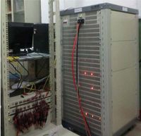
|
Download:
|
| Fig. 11 Battery test equipment. | |
A fractional order estimator is designed to estimate SOC of the battery.
For the common integer order system, Kalman filter approach is widely used to estimate the parameters of the system.
Hence, fractional order Kalman filter (FKF)[21] is selected to estimate the SOC of the battery.
The process can be described as:
1) $k=0$
The Kalman filter is initialized with the best available information of state and error covariance. The initialized value of state estimation and error covariance are expressed as: the covariance matrices of process noise $Q$, the covariance matrices of measurement noise $R$, the initialized system state $\hat{x}_{0}$, and the covariance matrices of initialized system state $P_{0}$ $=$ $E[(\hat{x}_{0}-x_{0})(\hat{x}_{0}-x_{0})^{\rm T}]$.
2) $k=1$, $2$, $\ldots$
State estimation propagation
| \begin{align} \label{eq:23} \tilde{x}_{k}=A_{d}x_{k-1}+B_{d}I_{k}-\sum_{j=1}^k\gamma_{j}\left(\begin{array}{c}N\\j\end{array}\right)x_{k-j}. \end{align} | (23) |
Error covariance propagation
| \begin{align} \label{eq:24} \tilde{P}_{k}=(A_{d}+N_{1})P_{k-1}+Q_{k-1}+\sum_{j=2}^kN_{j}P_{k-j}N_{j}^{\rm T}. \end{align} | (24) |
Kalman gain update
| \begin{align} \label{eq:25} K_{k}=\tilde{P}_{k}C^{\rm T}(C\tilde{P}_{k}C^{\rm T}+R_{k}). \end{align} | (25) |
State estimation update
| \begin{align} \label{eq:26} \hat{x}_{k}=\tilde{x}_{k}+K_{k}(y_{k}-C\tilde{x}_{k}). \end{align} | (26) |
Error covariance update
| \begin{align} \label{eq:27} P_{k}=(1-K_{k}C)\tilde{P}_{k}. \end{align} | (27) |
3) Save the estimated state and covariance for further iteration.
4) Separate the system state, and we will get SOC timely.
The current profile shown in Fig. 12 is employed as validation scenario. Under this condition, fractional Kalman filter and Kalman filter (KF) are used to estimate terminal voltage and SOC of battery. Both the measured terminal voltage and model terminal voltage are shown in Fig. 13. From Fig. 13, we can see the battery is tested in full SOC range (i.e., terminal voltage from 2.0 V to 3.6 V), and both the terminal voltage estimated by FKF and KF can trace the measured terminal voltage well, but the FKF results are more precise than the KF ones.

|
Download:
|
| Fig. 12 Current profile for SOC estimation. | |

|
Download:
|
| Fig. 13 Terminal voltage profile for SOC estimation. | |
SOC estimation and SOC estimation error curves are shown in Fig. 14 and Fig. 15, respectively. From Fig. 15 we will see, at the beginning of battery charging, the FKF estimation error is almost the same as KF estimation error. And with further charging of battery, precision of FKF will rise gradually while precision of KF gets worse. At the late charging period, both the FKF and KF error are increasing, but the FKF estimation error is always smaller than the KF one. In the whole test, the error of FKF can be reduced up to max 0.5% SOC, while the error of KF reaches 3%.

|
Download:
|
| Fig. 14 SOC estimation. | |

|
Download:
|
| Fig. 15 SOC estimation error. | |
Based on the analysis of the impedance spectra, a simplified battery fractional-order model is derived. A new identification method is presented to identify the orders of the states and parameters based on the fractional-order system. The fractional Kalman filter is utilized to estimate the SOC of the lithium-ion battery based on the fractional-order model. The simulation results show the SOC estimation with fractional Kalman filter is consistent with expectations. However just one battery is tested in the paper, battery pack will be tested in further study.
| [1] | Wang Y, Zhang C, Chen Z. A method for joint estimation of stateof-charge and available energy of LiFePO 4 batteries. Applied Energy, 2014, 135: 81-87 |
| [2] | Kim D, Koo K, Jeong J J, Goh T, Sang W K. Second-order discretetime sliding mode observer for state of charge determination based on a dynamic resistance Li-ion battery model. Energies, 2013, 6(10): 5538-5551 |
| [3] | Chen X, Shen W X, Cao Z, Kapoor A. Sliding mode observer for state of charge estimation based on battery equivalent circuit in electric vehicles. Australian Journal of Electrical and Electronics Engineering, 2012, 9(3): 225-234 |
| [4] | Li D, Ouyang J, Li H, Wan J F. State of charge estimation for LiMn 2O 4 power battery based on strong tracking sigma point Kalman filter. Journal of Power Sources, 2015, 279: 439-449 |
| [5] | He Ling-Na, Wang Yun-Hong. SOC estimation based on improved sampling point Kalman filter for mine-used battery. Journal of Mechanical and Electrical Engineering, 2014, 31(9): 1213-1217 (in Chinese) |
| [6] | Wang Y J, Zhang C B, Chen Z H. A method for state-of-charge estimation of LiFePO 4 batteries at dynamic currents and temperatures using particle filter. Journal of Power Sources, 2015, 279: 306-311 |
| [7] | Li J H, Barillas J K, Guenther C, Danzer M A. Multicell state estimation using variation based sequential Monte Carlo filter for automotive battery packs. Journal of Power Sources, 2015, 277: 95-103 |
| [8] | Lu L G, Han X B, Li J Q, Hua J F, Ouyang M G. A review on the key issues for Lithium-ion battery management in electric vehicles. Journal of Power Sources, 2013, 226: 272-288 |
| [9] | Deng Li-Wei, Song Shen-Min. Synchronization of fractional order hyperchaotic systems based on output feedback sliding mode control. Acta Automatica Sinica, 2014, 40(11): 2420-2427 (in Chinese) |
| [10] | Sadli I, Urbain M, Hinaje M, Martin J P, Raëel S, Davat B. Contributions of fractional differentiation to the modelling of electric double layer capacitance. Energy Conversion and Management, 2010, 51(12): 2993-2999 |
| [11] | Fairweather A J, Foster M P, Stone D A. Battery parameter identification with pseudo random binary sequence excitation (PRBS). Journal of Power Sources, 2011, 196(22): 9398-9406 |
| [12] | Sabatier J, Cugnet M, Laruelle S, Grugeon S, Sahut B, Oustaloup A, Tarascon J M. A fractional order model for lead-acid battery crankability estimation. Communications in Nonlinear Science and Numerical Simulation, 2010, 15(5): 1308-1317 |
| [13] | Sabatier J, Aoun M, Oustaloup A, Grégoire G, Ragot F, Roy P. Fractional system identification for lead acid battery state of charge estimation. Signal Processing, 2006, 86(10): 2645-2657 |
| [14] | Wu H J, Yuan S F, Yin C L. A Lithium-Ion battery fractional order state space model and its time domain system identification. In: Proceedings of the 2012 FISITA World Automotive Congress. Berlin Heidelberg: Springer, 2013, 192: 795-805 |
| [15] | Luo Y F, Gong C S A, Chang L X, Liu Y H. AC impedance technique for dynamic and static state of charge analysis for Li-ion battery. In: Proceedings of the 17th IEEE International Symposium on Consumer Electronics (ISCE). Hsinchu, China: IEEE, 2013: 9-10 |
| [16] | Eddahech A, Briat O, Bertrand N, Delétage J Y, Vinassa J M. Behavior and state-of-health monitoring of Li-ion batteries using impedance spectroscopy and recurrent neural networks. International Journal of Electrical Power and Energy Systems, 2012, 42(1): 487-494 |
| [17] | Barsoukov E, Macdonald J R. Impedance Spectroscopy: Theory, Experiment, and Applications (2nd edition). Hoboken, NJ: Wiley-Interscience, 2005. |
| [18] | Guermah S, Djennoune S, Bettayeb M. Discrete-time fractional-order systems: modeling and stability issues. Advances in Discrete Time Systems. INTECH Open Access Publisher, 2012. |
| [19] | Guermah S, Djennoune S, Bettayeb M. Controllability and observability of linear discrete-time fractional-order systems. International Journal of Applied Mathematics and Computer Science, 2008, 18(2): 213-222 |
| [20] | Victor S, Malti R, Garnier H, Oustaloup A. Parameter and differentiation order estimation in fractional models. Automatica, 2013, 49(4): 926-935 |
| [21] | Sierociuk D, Dzieliński A. Fractional Kalman filter algorithm for the states, parameters and order of fractional system estimation. International Journal of Applied Mathematics and Computer Science, 2006, 16(1): 129-140 |
 2016, Vol.3


