Direct Trajectory Optimization and Costate Estimation of Infinite-horizon Optimal Control Problems Using Collocation at the Flipped Legendre-Gauss-Radau Points
Ⅰ. INTRODUCTION
Finite-horizon optimal control problems are
fundamental problems in optimal control theory and application.
Over the last three decades,many reliable and efficient numerical
methods have been devised and employed to solve such problems,
which,in general,can be grouped into two major categories:
indirect methods and direct methods. The indirect approach uses
the calculus of variations to derive the first-order necessary
optimality conditions which are then solved to determine candidate
optimal solutions. The direct approach transcribes the original
problem to a nonlinear programming problem (NLP) which is then
solved to obtain optimal solutions. In recent years,a subset of
direct methods that have seen extensive use in the numerical
solution of finite-horizon optimal control problems are
pseudospectral methods[1, 2, 3, 4, 5, 6, 7]. The main advantages of
pseudospectral methods over other direct methods are the spectral
convergence rate and the costate estimation capacity.
The basic principle of pseudospectral methods is to approximate the
state using a set of basis functions and the differential-algebraic
constraints are enforced at specified set of collocation points. The
basis functions are typically Lagrange interpolating polynomials and
the collocation points are commonly chosen as Legendre-Gauss-Lobatto
(LGL),Legendre-Gauss (LG),and Legendre-Gauss-Radau (LGR) points
with the corresponding methods being called as Lobatto
pseudospectral method (LPM)[1, 2, 3],Gauss pseudospectral method
(GPM)[4, 5],and Radau pseudospectral method (RPM)[6, 7],
respectively. It is noted that the LGR points are defined on the
half-open interval $[-1,+1)$ or $(-1,+1]$,and thus,can be
classified into standard LGR and flipped LGR (FLGR) points,
respectively. In this paper we adopt the term flipped RPM (FRPM) for
the collocation at the FLGR points while reserving the RPM for the
collocation at the standard LGR points. It was shown in [8] that,
similar to the RPM,the FRPM is also an implicit integration method
with the differential and integral forms being equivalent,and
therefore,has the ability to obtain highly accurate discrete
approximation. Furthermore,the FRPM has the numerical stability
advantage over the RPM in that it is L-stable[9] and also
algebraically stable[10].
More recently,pseudospectral methods such as GPM[11] and
RPM[6, 11, 12] have also been used to solve infinite-horizon
optimal control problems. At their core,a change of variables is
used to transform the semi-infinite domain to the finite domain,and
as a result,an infinite-horizon problem is converted into a
finite-horizon problem. Attracted by the aforementioned high
accuracy and numerical stability advantages of the FRPM,in this
paper we extend the FRPM to solve infinite-horizon optimal control
problems. Specifically,the main contributions of this work are as
follows. First,in order to avoid the singularity~ of collocation~
at the point $+1$ associated with the transformation presented in [11] which
maps the scaled right half-open interval $\tau\in[-1,+1)$ to the
increasing time interval $t\in[0,+\infty)$,a new smooth,strictly
monotonic-decreasing transformation is proposed to map the scaled
left half-open interval $\tau\in(-1,+1]$ to the descending time
interval $t\in(+\infty,0]$. Second,the costate and constraint
multiplier estimates for the FRPM are derived in detail by comparing
the discretized necessary optimality conditions of a finite-horizon
optimal control problem with the Karush-Kuhn-Tucker (KKT) conditions
of the NLP resulting from collocation. As a result,the state and
costate approximation on the entire horizon,including the
approximation at $t=+\infty$,can be accurately obtained from the
solutions of the NLP with good numerical stability.
The rest of this paper is organized as follows. The
infinite-horizon optimal control problem and the corresponding
necessary optimality conditions are reviewed in Section Ⅱ . In
Section Ⅲ ,the implementation details of the FRPM are presented,
and the costate estimates are derived in detail in Section Ⅳ. The
numerical results from the FRPM are shown in Section Ⅴ. Finally,
Section Ⅵ contains some concluding remarks.
Ⅱ. SCALED OPTIMAL CONTROL PROBLEM AND NECESSARY OPTIMALITY CONDITIONS
A. Scaled Optimal Control Problem
Consider the following infinite-horizon optimal control problem.
Determine the state,${\pmb x}(t)R^{n_x}$,and control,
${\pmb u}(t)$ $\in$ $R^{n_u}$,on the time interval
$t\in[0,+\infty)$ that minimize the cost functional
|
\begin{array}{l}\
J=\int_0^{\infty}g({\pmb x}(t),{\pmb u}(t),t)\rm{d} t R,
\end{array}
|
(1)
|
subject to the dynamic constraints
|
\begin{equation}
\dot{{\pmb x}}(t)={\pmb f}({\pmb x}(t),{\pmb u}(t),t) R^{n_x},
\end{equation}
|
(2)
|
the inequality path constraints
|
\begin{equation}
{\pmb c}({\pmb x}(t),{\pmb u}(t),t)\leq{\pmb 0} R^{n_c},
\end{equation}
|
(3)
|
and the boundary conditions
|
\begin{equation} \label{E:INFOCP1_bc}
{\pmb b}({\pmb x}(0))={\pmb 0} R^{n_b}.
\end{equation}
|
(4)
|
In [11],a general change of variables $t=\phi(\tau)$ where $\phi$
is smooth,strictly monotonically increasing function of $\tau$ is
used to map the scaled right half-open interval $[-1,+1)$ to the
increasing time interval $[0,+\infty)$. As a result,the
infinite-horizon problem is converted into a finite-horizon problem
which is then discretized using collocation at the LG or LGR points.
However,this popular transformation cannot be used for the FLGR
points due to the singularity of collocation at the point $+1$. In
this work,a new general transformation $t=\zeta(\tau)$ where
$\zeta$ is a smooth,strictly monotonically decreasing function of
$\tau$ is proposed to map the scaled left half-open interval $\tau$
$\in$ $(-1$,$+1]$ to the descending time interval
$t\in(+\infty,0]$,and three examples of such a function are
|
\begin{array}{l}
\zeta_a(\tau)=\frac{1-\tau}{1+\tau},\\
\end{array}
|
(5a)
|
|
\begin{array}{l}
\zeta_b(\tau)=\ln\left(\frac{2}{1+\tau}\right),
\end{array}
|
(5b)
|
|
\begin{array}{l}
\zeta_c(\tau)=\ln\left(\frac{4}{(1+\tau)^2}\right),
\end{array}
|
(5c)
|
with the corresponding derivatives
|
\begin{array}{l}
\zeta_a'(\tau)=\frac{\rm{d}\zeta_a(\tau)}{\rm{d}\tau}=-\frac{2}{(1+\tau)^2},\label{E:tau2t_derivative1}
\end{array}
|
(6a)
|
|
\begin{array}{l}
\zeta_b'(\tau)=\frac{\rm{d}\zeta_b(\tau)}{\rm{d}\tau}=-\frac{1}{1+\tau} ,\label{E:tau2t_derivative2}
\end{array}
|
(6b)
|
|
\begin{array}{l}
\zeta_c'(\tau)=\frac{\rm{d}\zeta_c(\tau)}{\rm{d}\tau}=-\frac{2}{1+\tau}. \label{E:tau2t_derivative3}
\end{array}
|
(6c)
|
Using the new transformation $t=\zeta(\tau)$ and its derivative
$\frac{\rm{d} t}{\rm{d}\tau}=\zeta'(\tau)$,the infinite-horizon optimal
control problem of (1)-(4) is then converted into the scaled
finite-horizon optimal control problem in terms of the variable
$\tau$ as follows. Determine the state,${\pmb x}(\tau)\in{\bf
R}^{n_x}$,and control,${\pmb u}(\tau)R^{n_u}$,on the
scaled left half-open interval $\tau\in(-1,+1]$ that minimize the
cost functional
|
\begin{array}{l} \label{E:DIF_OCP_cost}
J=\int_{+1}^{-1}\zeta'(\tau)g({\pmb x}(\tau),{\pmb u}(\tau),\tau)\rm{d}\tau \notag
&\\ \quad =-\int_{-1}^{+1}\zeta'(\tau)g({\pmb x}(\tau),{\pmb u}(\tau),\tau)\rm{d}\tau \notag
&\\ =\int_{-1}^{+1}g^\zeta({\pmb x}(\tau),{\pmb u}(\tau),\tau)\rm{d}\tau R,
\end{array}
|
(7)
|
subject to the dynamic constraints
|
\begin{array}{l} \label{E:DIF_OCP_dc}
\dot{{\pmb x}}(\tau)=\zeta'(\tau){\pmb f}({\pmb x}(\tau),{\pmb u}(\tau),\tau) \notag
&\\={\pmb f}^\zeta({\pmb x}(\tau),{\pmb u}(\tau),\tau) R^{n_x},
\end{array}
|
(8)
|
the inequality path constraints
|
\begin{equation} \label{E:DIF_OCP_pc}
{\pmb c}({\pmb x}(\tau),{\pmb u}(\tau),\tau)\leq{\pmb 0} R^{n_c},
\end{equation}
|
(9)
|
and the boundary conditions
|
\begin{equation} \label{E:DIF_OCP_bc}
{\pmb b}({\pmb x}(+1))={\pmb 0} R^{n_b}.
\end{equation}
|
(10)
|
where
|
\begin{array}{l}
g^\zeta({\pmb x}(\tau),{\pmb u}(\tau),\tau)=-\zeta'(\tau)g({\pmb x}(\tau),{\pmb u}(\tau),\tau) ,
\end{array}
|
(11a)
|
|
\begin{array}{l}
{\pmb f}^\zeta({\pmb x}(\tau),{\pmb u}(\tau),\tau)=\zeta'(\tau){\pmb f}({\pmb x}(\tau),{\pmb u}(\tau),
\end{array}
|
(11b)
|
Equations (7)-(10) will be referred to as the scaled optimal control
problem which will be discretized using the FRPM in Section Ⅲ.
B. Necessary Optimality Conditions
The necessary optimality conditions of the above scaled optimal
control problem are found by applying the calculus of variations to
the augmented cost function,which is created by adjoining the
costate,${\pmb \lambda}(\tau)R^{n_x}$,the Lagrange
multipliers,${\pmb \mu}(\tau)$ $\in$ $R^{n_c}$ and ${\pmb
\nu}R^{n_b}$,as
|
\begin{array}{l}
J_a=-{\pmb \nu}^{\rm T}{\pmb b}+\int_{-1}^{+1}\bigg[g^\zeta-{\pmb \lambda}^{\rm T}
\Big(\dot{{\pmb x}}-{\pmb f}^\zeta\Big)-{\pmb \mu}^{\rm T}{\pmb c}\bigg]\rm{d}\tau \notag
&\\=-{\pmb \nu}^{\rm T}{\pmb b}+\int_{-1}^{+1}\bigg[\Big(g^\zeta+{\pmb \lambda}^{\rm T}
{\pmb f}^\zeta-{\pmb \mu}^{\rm T}{\pmb c}\Big)-{\pmb \lambda}^{\rm T}\dot{{\pmb
x}}\bigg]\rm{d}\tau.
\end{array}
|
(12)
|
The first-order variation of the augmented cost becomes
|
\begin{array}{l}
\delta J_a= -\delta{\pmb \nu}^{\rm T}{\pmb b}-{\pmb \nu}^{\rm T}\bigg(\frac{\partial{{\pmb b}}}{\partial{{\pmb x}(+1)}}\delta{\pmb x}(+1)\bigg) \notag
&\\ +\int_{-1}^{+1}\bigg[\bigg(\frac{\partial{g^\zeta}}{\partial{{\pmb x}}}\delta{\pmb x}+\frac{\partial{g^\zeta}}{\partial{{\pmb u}}}\delta{\pmb u}\bigg) \notag
&\\ +{\pmb \lambda}^{\rm T}\bigg(\frac{\partial{{\pmb f}^\zeta}}{\partial{{\pmb x}}}\delta{\pmb x}+\frac{\partial{{\pmb f}^\zeta}}{\partial{{\pmb u}}}\delta{\pmb u}\bigg) \notag
&\\ -{\pmb \mu}^{\rm T}\bigg(\frac{\partial{{\pmb c}}}{\partial{{\pmb x}}}\delta{\pmb x}+\frac{\partial{{\pmb c}}}{\partial{{\pmb u}}}\delta{\pmb u}\bigg) \notag
&\\ -{\pmb \lambda}^{\rm T}\delta\dot{{\pmb x}}-\delta{\pmb \lambda}^{\rm T}\Big(\dot{{\pmb x}}-{\pmb f}^\zeta\Big)-\delta{\pmb \mu}^{\rm T}{\pmb
c}\bigg]\rm{d}\tau,
\end{array}
|
(13)
|
where
|
\begin{array}{l} \label{E:DIF_OCP_LambdaX_}
&\\ int_{-1}^{+1}-{\pmb \lambda}^{\rm T}\delta\dot{{\pmb x}} \rm{d}\tau=-{\pmb \lambda}^{\rm T}(+1)\delta{\pmb x}(+1)\notag
&\\ \qquad+{\pmb \lambda}^{\rm T}(-1)\delta{\pmb x}(-1)+\int_{-1}^{+1}\dot{{\pmb \lambda}}^{\rm T}\delta{\pmb
x}\rm{d}\tau.
\end{array}
|
(14)
|
Substituting (14) into (13) and collecting like terms yields
|
\begin{array}{l} \label{E:DIF_OCP_DeltaJ_}
\delta J_a= -\delta{\pmb \nu}^{\rm T}{\pmb b}+{\pmb \lambda}^{\rm T}(-1)\delta{\pmb x}(-1)\notag
&\\ -\bigg({\pmb \nu}^{\rm T}\frac{\partial{{\pmb b}}}{\partial{{\pmb x}(+1)}}+{\pmb \lambda}^{\rm T}(+1)\bigg)\delta{\pmb x}(+1)\notag
&\\ +\int_{-1}^{+1}\bigg[\bigg(\dot{{\pmb \lambda}}^{\rm T}+\bigg(\frac{\partial{g^\zeta}}
{\partial{{\pmb x}}}+{\pmb \lambda}^{\rm T}\frac{\partial{{\pmb f}^\zeta}}{\partial{{\pmb x}}}-{\pmb \mu}^{\rm T}\frac{\partial{{\pmb c}}}{\partial{{\pmb x}}}\bigg)\bigg)\delta{\pmb x} \notag
&\\ +\bigg(\frac{\partial{g^\zeta}}{\partial{{\pmb u}}}+{\pmb \lambda}^{\rm T}\frac{\partial{{\pmb f}^\zeta}}
{\partial{{\pmb u}}}-{\pmb \mu}^{\rm T}\frac{\partial{{\pmb c}}}{\partial{{\pmb u}}}\bigg)\delta{\pmb u}\notag
&\\ -\delta{\pmb \lambda}^{\rm T}\Big(\dot{{\pmb x}}-{\pmb f}^\zeta\Big)-\delta{\pmb \mu}^{\rm T}{\pmb
c}\bigg]\rm{d}\tau.
\end{array}
|
(15)
|
Setting equal to zero the coefficients of the independent
increments,$\delta{\pmb \lambda}$,$\delta{\pmb x}$,$\delta{\pmb
u}$,$\delta{\pmb \mu}$,$\delta{\pmb \nu}$,$\delta{\pmb x}(-1)$
and $\delta{\pmb x}(+1)$,results in the following necessary
optimality conditions:
|
\begin{array}{l}
\dot{{\pmb x}}^{\rm T}(\tau)={\pmb f}^{\zeta^{\rm T}}=\frac{\partial{\mathcal{H}}}{\partial{{\pmb \lambda}}},\label{E:DIF_OCP_oc1}
\end{array}
|
(16a)
|
|
\begin{array}{l}
\dot{{\pmb \lambda}}^{\rm T}(\tau)=-\bigg(\frac{\partial{g^\zeta}}{\partial{{\pmb x}}}+{\pmb \lambda}^{\rm T}\frac{\partial{{\pmb f}^\zeta}}{\partial{{\pmb x}}}-{\pmb \mu}^{\rm T}\frac{\partial{{\pmb c}}}{\partial{{\pmb x}}}\bigg)=-\frac{\partial{\mathcal{H}}}{\partial{{\pmb x}}},
\end{array}
|
(16b)
|
|
\begin{array}{l}
\frac{\partial{g^\zeta}}{\partial{{\pmb u}}}+{\pmb \lambda}^{\rm T}\frac{\partial{{\pmb f}^\zeta}}{\partial{{\pmb u}}}-{\pmb \mu}^{\rm T}\frac{\partial{{\pmb c}}}{\partial{{\pmb u}}}=\frac{\partial{\mathcal{H}}}{\partial{{\pmb u}}}={\pmb 0}^{\rm T},
\end{array}
|
(16c)
|
|
\begin{array}{l}
\begin{cases}
{\pmb c}^{\rm T}\leq{\pmb 0}^{\rm T},
\mu_j=0,&\\ when c_j<0,
\mu_j\leq0,&\\ when c_j=0,
\end{cases}
\end{array}
|
(16d)
|
|
\begin{array}{l}
{\pmb b}^{\rm T}({\pmb x}(+1))={\pmb 0}^{\rm T},
\end{array}
|
(16e)
|
|
\begin{array}{l}
{\pmb \lambda}^{\rm T}(-1)={\pmb 0}^{\rm T},
\end{array}
|
(16f)
|
|
\begin{array}{l}
{\pmb \lambda}^{\rm T}(+1)=-{\pmb \nu}^{\rm T}\frac{\partial{{\pmb b}}}{\partial{{\pmb
x}(+1)}},
\end{array}
|
(16g)
|
where $\mathcal{H}$ is the Hamiltonian,defined as
|
\begin{array}{l}
\mathcal{H}:=\mathcal{H}({\pmb x}(\tau),{\pmb u}(\tau),{\pmb \lambda}(\tau),{\pmb \mu}(\tau),\tau)\notag
&\\ :=g^\zeta+{\pmb \lambda}^{\rm T}{\pmb f}^\zeta-{\pmb \mu}^{\rm T}{\pmb
c}.
\end{array}
|
(17)
|
The necessary optimality conditions of (16a)-(16g) result in what is
commonly referred to as the Hamiltonian boundary-value problem,
which must be solved numerically to obtain the optimal solution of
the original optimal control problem.
Remark 1. It can be seen from (5) that for the change of
variables $t=\zeta(\tau)$,the costate of the original
infinite-horizon optimal control problem is actually the negative
of the costate of the corresponding scaled optimal control problem resulting from transformation,i.e.,
|
\begin{equation} \label{E:CostatesZetaTransformation}
{\pmb \lambda}(t)=-{\pmb \lambda}^\zeta(t).
\end{equation}
|
(18)
|
Ⅲ. FLIPPED RADAU PSEUDOSPECTRAL METHOD
In the FRPM,the state is approximated using a basis of $N$ $+$ $1$
Lagrange interpolating polynomials as follows:
|
\begin{equation} \label{E:StateApprox}
{\pmb x}(\tau)\approx{\pmb x}^N(\tau)=\sum_{i=0}^N{\pmb x}
(\tau_i)\mathcal{L}_i(\tau)=\sum_{i=0}^N\mathcal{L}_i(\tau){\pmb
x}(\tau_i),
\end{equation}
|
(19)
|
where $\{\tau_i\}_{i=0}^N$ are the state interpolation points
containing the start point $\tau_0:=-1$ and the FLGR points,and
$\{\mathcal{L}_i(\tau)\}_{i=0}^N$ are the $N$th-order Lagrange
interpolating polynomials,defined as
|
\begin{equation} \label{E:LagrangeDef}
\mathcal{L}_i(\tau):=\prod\limits_{j=0,j\neq i}^N\frac{\tau-\tau_j}{\tau_i-\tau_j},\quad i=0,1,...,
N,
\end{equation}
|
(20)
|
or equivalently represented in barycentric form[13]
|
\begin{equation} \label{E:LagrangeBary}
\mathcal{L}_i(\tau)=\dfrac{\dfrac{\xi_i}{\tau-\tau_i}}{{\displaystyle\sum_{j=0}^N\dfrac{\xi_j}{\tau-\tau_j}}},\quad i=0,1,...,
N,
\end{equation}
|
(21)
|
where $\{\xi_i\}_{i=0}^N$ are the barycentric weights,defined
as[13]
|
\begin{equation} \label{E:BaryWeights1}
\xi_i:=\frac{1}{\prod\limits_{j=0,j\neq i}^N(\tau_i-\tau_j)},\quad i=0,1,...,
N.
\end{equation}
|
(22)
|
Although equivalent,the barycentric Lagrange interpolation has
significant advantages over the classic Lagrange interpolation in
terms of the numerical stability and computational
efficiency[13]. It can be seen from (20) that
$\{\mathcal{L}_i(\tau)\}_{i=0}^N$ satisfy the Kronecker property
|
\begin{equation} \label{E:LagrangeProp}
\mathcal{L}_i(\tau_j)=\begin{cases}
1,&j=i \\
0,&j\neq i
\end{cases},\quad i,j=0,1,...,
N.
\end{equation}
|
(23)
|
Furthermore,(19) and (23) imply that ${\pmb x}^N(\tau_i)={\pmb
x}(\tau_i)$,$i=0,$ $1,...,N$. The time derivative of the state
approximation of (19) is given by
|
\begin{equation} \label{E:StateDerivApprox}
\dot{{\pmb x}}(\tau)\approx\dot{{\pmb x}}^N(\tau)=\sum_{i=0}^N{\pmb x}(\tau_i)\dot{\mathcal{L}}_i(\tau)=\sum_{i=0}^N\dot{\mathcal{L}}_i(\tau){\pmb
x}(\tau_i).
\end{equation}
|
(24)
|
Using (24),the dynamic constraints of (8) are then collocated at
the $N$ FLGR points $\{\tau_k\}_{k=1}^N$ as
|
\begin{equation} \label{E:NLP_dc}
\sum_{i=0}^ND_{ki}{\pmb x}_i-{\pmb f}^\zeta({\pmb x}_k,{\pmb u}_k,\tau_k)={\pmb 0},\quad k=1,2,...,
N,
\end{equation}
|
(25)
|
where $D_{ki}:=\dot{\mathcal{L}}_i(\tau_k)\in{\bf
R}^{N\times(N+1)}$,$k=1,2,...,N$,$i=0,$ $1,...,N$ is the
FLGR pseudospectral differentiation matrix,${\pmb x}_i:={\pmb
x}(\tau_i)={\pmb x}^N(\tau_i)$,$i=0,1,...,N$,and ${\pmb
u}_k:={\pmb u}(\tau_k)$,$k=1,2,...,N$. Note that the dynamic
constraints are not collocated at the initial point $\tau_0$. It can
be seen from (25) that the accuracy and robustness of the
approximation to the dynamic constraints are highly dependent upon
that of the matrix $D$. One straightforward way to compute $D$ is
via the definition of the Lagrange interpolating polynomials. Using
(20),the time derivatives of $\{\mathcal{L}_i(\tau)\}_{i=0}^N$ can
be written as
|
\begin{equation}
\dot{\mathcal{L}}_i(\tau)=\sum_{l=0,l\neq i}^N\frac{\prod\limits_{j=0,j\neq i,l}^N(\tau-\tau_j)}{\prod\limits_{j=0,j\neq i}^N(\tau_i-\tau_j)},\quad i=0,1,...,
N.
\end{equation}
|
(26)
|
$D$ is then given as
|
\begin{equation} \label{E:Dmatrix}
D_{ki}=\dot{\mathcal{L}}_i(\tau_k)=\sum_{l=0,l\neq i}^N\frac{\prod\limits_{j=0,j\neq i,l}^N(\tau_k-\tau_j)}
{\prod\limits_{j=0,j\neq i}^N(\tau_i-\tau_j)}.
\end{equation}
|
(27)
|
It can be seen from (27) that the direct approach to calculate $D$
is tedious,error-prone,and sometimes impossible due to numerical
difficulties. In order to alleviate the computational error and
improve the numerical stability and computational efficiency,the
barycentric form of (21) is adopted to calculate $D$ as
follows[13]:
|
\begin{equation} \label{E:DmatrixBary}
D_{ki}=\begin{cases}
\dfrac{\frac{\xi_i}{\xi_k}}{\tau_k-\tau_i},&k\neq i,
\\[4mm]
-\sum\limits_{j=0,j\neq k}^ND_{kj},&k=i,
\end{cases}
\end{equation}
|
(28)
|
where the second row of (28) arises from the fact that the
derivative of a constant function should be zero,or in other words,
the $\sum $ of all elements of $D$ in each row should be zero. The
advantages of (28) over (27) from the point of view of numerical
stability are discussed in [14]. Next,the cost functional of (7) is
approximated using the FLGR quadrature as
|
\begin{equation} \label{E:NLP_cost}
J^N=\sum_{k=1}^N\omega_kg^\zeta({\pmb x}_k,{\pmb u}_k,
\tau_k).
\end{equation}
|
(29)
|
Furthermore,the path constraints of (9) are
evaluated at the FLGR points as
|
\begin{equation} \label{E:NLP_pc}
{\pmb c}({\pmb x}_k,{\pmb u}_k,\tau_k)\leq{\pmb 0},\quad k=1,2,...,
N.
\end{equation}
|
(30)
|
Finally,the boundary conditions of (10) are approximated at the
boundary points as
|
\begin{equation} \label{E:NLP_bc}
{\pmb b}({\pmb x}_N)={\pmb 0}.
\end{equation}
|
(31)
|
The cost function of (29) along with the algebraic constraints of
(25),(30) and (31) defines an NLP which is the FLGR pseudospectral
approximation to the scaled optimal control problem.
Ⅳ. COSTATE ESTIMATION USING THE FRPM
A. KKT Conditions of the NLP
The solution to the NLP must satisfy a set of first-order
optimality conditions called the KKT conditions,which can be
obtained using the augmented cost function with the Lagrange
multipliers $\{\tilde{{\pmb \lambda}}_k\in{\bf
R}^{n_x}\}_{k=1}^N$,$\{\tilde{{\pmb \mu}}_k\in{\bf
R}^{n_c}\}_{k=1}^N$ and $\tilde{{\pmb \nu}}R^{n_b}$ as
|
\begin{array}{l}
J_a^N= \sum_{k=1}^N\omega_kg^\zeta({\pmb x}_k,{\pmb u}_k,\tau_k)-\tilde{{\pmb \nu}}^{\rm T}{\pmb b}
({\pmb x}_N)-\!\sum_{k=1}^N\tilde{{\pmb \mu}}_k^{\rm T}{\pmb c}({\pmb x}_k,{\pmb u}_k,\tau_k)\notag
&\\ -\sum_{k=1}^N\tilde{{\pmb \lambda}}_k^{\rm T}\Bigg(\sum_{i=0}^ND_{ki}{\pmb x}_i-{\pmb f}^\zeta({\pmb x}_k,{\pmb u}_k,\tau_k)\Bigg)\notag
&\\ = -\tilde{{\pmb \nu}}^{\rm T}{\pmb b}({\pmb x}_N)-\sum_{i=1}^N\tilde{{\pmb \lambda}}_i^{\rm T}
\sum_{k=1}^ND_{ik}{\pmb x}_k-\sum_{i=1}^N\tilde{{\pmb \lambda}}_i^{\rm T}D_{i0}{\pmb x}_0\notag
&\\ +\sum_{k=1}^N\omega_kg^\zeta_k+\sum_{k=1}^N\tilde{{\pmb \lambda}}_k^{\rm T}
{\pmb f}^\zeta_k-\sum_{k=1}^N\tilde{{\pmb \mu}}_k^{\rm T}{\pmb
c}_k,
\end{array}
|
(32)
|
where $g^\zeta_k:= g^\zeta({\pmb x}_k,{\pmb u}_k,\tau_k)$,${\pmb
f}^\zeta_k:={\pmb f}^\zeta({\pmb x}_k,{\pmb u}_k,\tau_k)$ and
${\pmb c}_k:={\pmb c}({\pmb x}_k,{\pmb u}_k,\tau_k)$. Setting
equal to zero the partial derivatives of the augmented cost function
with respect to $\{\tilde{{\pmb \lambda}}_k\}_{k=1}^N$,$\{{\pmb
x}_k\}_{k=1}^N$,$\{{\pmb u}_k\}_{k=1}^N$,$\{\tilde{{\pmb
\mu}}_k\}_{k=1}^N$,$\tilde{{\pmb \nu}}$ and ${\pmb x}_0$ results in
the following KKT conditions:
|
\begin{array}{l}
\sum_{i=0}^ND_{ki}{\pmb x}_i^{\rm T}={\pmb f}^{\zeta^{\rm T}}_k,
\end{array}
|
(33a)
|
|
\begin{array}{l}
\begin{split} \label{E:NLP_KKT2}
-\sum_{i=1}^N\tilde{{\pmb \lambda}}_i^{\rm T}\frac{D_{ik}}{\omega_k}-\frac{\delta_{kN}}{\omega_N}
\Bigg(\tilde{{\pmb \nu}}^{\rm T}\frac{\partial{{\pmb b}}}{\partial{{\pmb x}_N}}\Bigg)
&\\ = -\Bigg(\frac{\partial{g^\zeta_k}}{\partial{{\pmb x}_k}} +
\frac{\tilde{{\pmb \lambda}}_k^{\rm T}}{\omega_k}\frac{\partial{{\pmb f}^\zeta_k}}
{\partial{{\pmb x}_k}}-\frac{\tilde{{\pmb \mu}}_k^{\rm T}}{\omega_k}\frac{\partial{{\pmb c}_k}}{\partial{{\pmb x}_k}}\Bigg)=-\frac{\partial{\tilde{\mathcal{H}}_k}}{\partial{{\pmb
x}_k}},
\end{split}
\end{array}
|
(33b)
|
|
\begin{array}{l}
\frac{\partial{g^\zeta_k}}{\partial{{\pmb u}_k}}+\frac{\tilde{{\pmb \lambda}}_k^{\rm T}}{\omega_k}
\frac{\partial{{\pmb f}^\zeta_k}}{\partial{{\pmb u}_k}}-\frac{\tilde{{\pmb \mu}}_k^{\rm T}}
{\omega_k}\frac{\partial{{\pmb c}_k}}{\partial{{\pmb u}_k}}=\frac{\partial{\tilde{\mathcal{H}}_k}}
{\partial{{\pmb u}_k}}={\pmb 0}^{\rm T},
\end{array}
|
(33c)
|
|
\begin{array}{l}
{\pmb c}_k^{\rm T}\leq{\pmb 0}^{\rm T},
\tilde{\mu}_{jk}=0,&\\ when c_{jk} < 0 ,
\tilde{\mu}_{jk}\leq0,
&\\ when c_{jk}=0,
\end{array}
|
(33d)
|
|
\begin{array}{l}
{\pmb b}^{\rm T}({\pmb x}_N)={\pmb 0}^{\rm T},
\end{array}
|
(33e)
|
|
\begin{array}{l}
\tilde{{\pmb \lambda}}_0^{\rm T}:=-\sum_{i=1}^ND_{i0}\tilde{{\pmb \lambda}}_i^{\rm T}={\pmb 0}^{\rm T},\label{E:NLP_KKT6}
\end{array}
|
(33f)
|
where
|
\begin{array}{l}
\tilde{\mathcal{H}}_k:=\tilde{\mathcal{H}}\left({\pmb x}_k,{\pmb u}_k,\tilde{{\pmb \lambda}}_k,\tilde{{\pmb \mu}}_k,\tau_k\right)\notag
&\\ :=g^\zeta_k+\frac{\tilde{{\pmb \lambda}}^{\rm T}_k}{\omega_k}{\pmb f}^\zeta_k-\frac{\tilde{{\pmb \mu}}^{\rm T}_k}{\omega_k}{\pmb
c}_k.
\end{array}
|
(34)
|
B. Flipped Radau Pseudospectral Discretization of the Necessary Optimality Conditions
In order to discretize the necessary optimality conditions of
(16a)-(16g) using pseudospectral methods,it is important to form an
appropriate approximation for the costate. In the FRPM,the costate
is approximated as follows:
|
\begin{equation} \label{E:CostateApprox}
{\pmb \lambda}(\tau)\approx{\pmb \lambda}^N(\tau)=\sum_{i=1}^N{\pmb \lambda}(\tau_i)\mathcal{L}_i^†(\tau)=\sum_{i=1}^N\mathcal{L}_i^†(\tau){\pmb \lambda}(\tau_i)
\end{equation}
|
(35)
|
where $\{\tau_i\}_{i=1}^N$ are the costate interpolation points
containing the FLGR points only,and
$\{\mathcal{L}_i^†(\tau)\}_{i=1}^N$ are the $(N-1)$th-order
Lagrange interpolating polynomials,defined as
|
\begin{equation} \label{E:LagrangeDef1}
\mathcal{L}_i^†(\tau):=\prod_{j=1,j\neq i}^N\frac{\tau-\tau_j}{\tau_i-\tau_j},\quad i=1,2,...,
N,
\end{equation}
|
(36)
|
from which it is seen that
|
\begin{equation}
\mathcal{L}_i^†(\tau_j)=\left\{ \begin{array}{l}
\begin{array}{*{20}{l}}
{1,}&{j = i}&{}
\end{array}\\
0,\;\;\;j \ne i
\end{array} \right.,\qquad i,j = 1,2,...,N.
\end{equation}
|
(37)
|
It is noteworthy here that the costate approximation differs from
the state approximation in that the costate approximation does not
include the start point. The time derivative of the costate
approximation is then given as
|
\begin{equation} \label{E:CostateDerivApprox}
\dot{{\pmb \lambda}}(\tau)\approx\dot{{\pmb \lambda}}^N(\tau)=\sum_{i=1}^N
{\pmb \lambda}(\tau_i)\dot{\mathcal{L}}_i^†(\tau)=\sum_{i=1}^N\dot{\mathcal{L}}_i^†(\tau){\pmb
\lambda}(\tau_i).
\end{equation}
|
(38)
|
In a manner similar to the state collocation,the costate is
collocated at the $N$ FLGR points $\{\tau_k\}_{k=1}^N$ as
|
\begin{array}{l}
\dot{{\pmb \lambda}}(\tau_k)\approx\dot{{\pmb \lambda}}^N(\tau_k)=\sum_{i=1}^N\dot{\mathcal{L}}_i^†(\tau_k){\pmb \lambda}(\tau_i)\notag
&\\ =\sum_{i=1}^ND_{ki}^†{\pmb \lambda}_i,\quad k=1,2,...,
N,
\end{array}
|
(39)
|
where $D_{ki}^†:=\dot{\mathcal{L}}_i^†(\tau_k)\in{\bf
R}^{N\times N}$,$k=1,2,...,N$,$i=1,2,$ $...,$ $N$ is the
adjoint FLGR pseudospectral differentiation matrix,and ${\pmb
\lambda}_i:={\pmb \lambda}(\tau_i)={\pmb \lambda}^N(\tau_i)$,$i=1,
2,...,N$. Furthermore,the costate approximation at the initial
time,${\pmb \lambda}_0={\pmb \lambda}^N(\tau_0)$ $=$
$\sum_{i=1}^N{\pmb \lambda}(\tau_i)\mathcal{L}_i^†(\tau_0)$,can
be obtained from the integration of (38) over the scaled interval
$\tau\in[-1,+1]$ as follows:
|
\begin{array}{l} \label{E:CostateApproxEnds}
{\pmb \lambda}_0 ={\pmb \lambda}_N-\int_{-1}^{+1}\dot{{\pmb \lambda}}^N(\tau)\rm{d}\tau\notag
&\\ ={\pmb \lambda}_N-\int_{-1}^{+1}\sum_{i=1}^N{\pmb \lambda}(\tau_i)\dot{\mathcal{L}}_i^†(\tau)\rm{d}\tau\notag
&\\ ={\pmb \lambda}_N-\sum_{i=1}^N{\pmb \lambda}_i\left(\int_{-1}^{+1}\dot{\mathcal{L}}_i^†(\tau)\rm{d}\tau\right)\notag
&\\ ={\pmb \lambda}_N-\sum_{i=1}^N{\pmb \lambda}_i\left(\sum_{k=1}^N\omega_k\dot{\mathcal{L}}_i^†(\tau_k)\right)\notag
&\\ ={\pmb \lambda}_N-\sum_{i=1}^N{\pmb \lambda}_i\left(\sum_{k=1}^N\omega_kD_{ki}^†\right)\notag
&\\ ={\pmb \lambda}_N-\sum_{k=1}^N\omega_k\sum_{i=1}^ND_{ki}^†{\pmb \lambda}_i
\end{array}
|
(40)
|
where the fourth row results from the FLGR quadrature rule which is
exact for polynomials of degree $2N-2$ or less with $N$ FLGR points.
Thus,using the state and costate approximation as given in (19),
(35) and (40),the necessary optimality conditions of (16a)-(16g)
are discretized as
|
\begin{array}{l}
\sum_{i=0}^ND_{ki}{\pmb x}_i^{\rm T}={\pmb f}^{\zeta^{\rm T}}_k,
\end{array}
|
(41a)
|
|
\begin{array}{l}
\sum_{i=1}^ND_{ki}^†{\pmb \lambda}_i^{\rm T}=\frac{\partial{\mathcal{H}}_k}{\partial{{\pmb x}_k}},
\end{array}
|
(41b)
|
|
\begin{array}{l}
\frac{\partial{\mathcal{H}}_k}{\partial{{\pmb u}_k}}={\pmb 0}^{\rm T} ,
\end{array}
|
(41c)
|
|
\begin{array}{l}
\begin{cases}
{\pmb c}_k^{\rm T}\leq{\pmb 0}^{\rm T},
\mu_{jk}=0,&\\ when c_{jk}<0,
\mu_{jk}\leq 0,&\\ when c_{jk}=0,
\end{cases}
\end{array}
|
(41d)
|
|
\begin{array}{l}
{\pmb b}^{\rm T}({\pmb x}_N)={\pmb 0}^{\rm T},
\end{array}
|
(41e)
|
|
\begin{array}{l}
{\pmb \lambda}_0^{\rm T}={\pmb 0}^{\rm T},
\end{array}
|
(41f)
|
|
\begin{array}{l}
{\pmb \lambda}_N^{\rm T}=-{\pmb \nu}^{\rm T}\frac{\partial{{\pmb b}}}{\partial{{\pmb x}_N}},
\end{array}
|
(41g)
|
|
\begin{array}{l}
{\pmb \lambda}_0^{\rm T}={\pmb \lambda}_N^{\rm T}-\sum_{k=1}^N\omega_k\sum_{i=1}^ND_{ki}^†{\pmb
\lambda}_i^{\rm T},
\end{array}
|
(41h)
|
where
|
\begin{array}{l}
\mathcal{H}_k:=\mathcal{H}({\pmb x}_k,{\pmb u}_k,{\pmb \lambda}_k,{\pmb \mu}_k,\tau_k)\notag
&\\ := g^\zeta_k+{\pmb \lambda}_k^{\rm T}{\pmb f}^\zeta_k-{\pmb \mu}_k^{\rm T}{\pmb
c}_k.
\end{array}
|
(42)
|
The solution to the above nonlinear algebraic equations is an
indirect solution to the scaled optimal control problem in (7)-(10).
C. Costate and Constraint Multiplier Estimates
The costate and constraint multiplier estimates of the Hamiltonian
boundary-value problem in (16a)-(16g) can be obtained from a
comparison of the discretized optimality conditions in Section IV-B
to the KKT conditions in Section IV-A. First,the matrices $D$ and
$D^†$ are related to one another as [8]
|
\begin{array}{l}
D_{NN}=-D_{NN}^†+\frac{1}{\omega_N},
&\\ \frac{D_{ik}}{\omega_k}=-\frac{D_{ki}^†}{\omega_i},\quad
\textrm{otherwise},
\end{array}
|
(43a)
|
|
\begin{array}{l}
D_{i0}=-\sum_{k=1}^ND_{ik},\quad i=1,2,...,N.
\end{array}
|
(43b)
|
To show this relationship,consider the following integration by
parts formula
|
\begin{array}{l}
int_{-1}^{+1}q^†(\tau)\dot{p}(\tau)\rm{d}\tau=p(+1)q^†(+1)\notag
&\\ \qquad-p(-1)q^†(-1)-\int_{-1}^{+1}p(\tau)\dot{q}^†(\tau)\rm{d}\tau,
\end{array}
|
(44)
|
where $p(\tau)$ is any interpolating polynomial of degree $N$ at the
interpolation points $\{\tau_i\}_{i=0}^N$,and $q^†(\tau)$ is any
interpolating polynomial of degree $N-1$ at the interpolation points
$\{\tau_i\}_{i=1}^N$. Thus,$q^†(\tau)\dot{p}(\tau)$ and
$p(\tau)\dot{q}^†(\tau)$ are polynomials of degree $2N$ $-$ $2$.
Since the FLGR quadrature is exact for polynomials of degree at most
$2N-2$ with $N$ FLGR points,the above integrals are then replaced
exactly by their quadrature equivalents as
|
\begin{array}{l}
\sum_{j=1}^N\omega_jq^†(\tau_j)\sum_{l=0}^ND_{jl}p(\tau_l)=p(+1)q^†(+1)\notag
&\\ \qquad-p(-1)q^†(-1)-\sum_{j=1}^N\omega_jp(\tau_j)\sum_{l=1}^ND_{jl}^†
q^†(\tau_l),
\end{array}
|
(45)
|
where $\dot{p}(\tau_j)=\sum_{l=0}^ND_{jl}p(\tau_l)$ and
$\dot{q}^†(\tau_j)=\sum_{l=1}^ND_{jl}^† q^†(\tau_l)$ are
used. Substituting the set of
$\{p(\tau)=\mathcal{L}_k(\tau)\}_{k=0}^N$ and $\{q^†(\tau)$
$=\mathcal{L}_i^†(\tau)\}_{i=1}^N$ into (45) gives
|
\begin{array}{l}
\sum_{j=1}^N\omega_j\mathcal{L}_i^†(\tau_j)\sum_{l=0}^ND_{jl}\mathcal{L}_k(\tau_l)=\mathcal{L}_k(+1)\mathcal{L}_i^†(+1)\notag
&\\ \quad\ \ -\mathcal{L}_k(-1)\mathcal{L}_i^†(-1)-\sum_{j=1}^N\omega_j\mathcal{L}_k(\tau_j)\sum_{l=1}^ND_{jl}^†\mathcal{L}_i^†(\tau_l),\notag
&\\ \qquad\qquad\qquad\qquad k=0,1,...,N,\ \ i=1,2,...,
N.
\end{array}
|
(46)
|
From (23) and (37),it can be seen that
|
\begin{array}{l}
\mathcal{L}_k(\tau_j)=\delta_{kj},\quad k,j=0,1,...,N,\notag
&\\ \mathcal{L}_i^†(\tau_j)=\delta_{ij},\quad i,j=1,2,...,
N.
\end{array}
|
(47)
|
Then,(46) reduces to
|
\begin{array}{l}
\sum_{j=1}^N\omega_j\delta_{ij}\sum_{l=1}^ND_{jl}\delta_{kl}=\delta_{kN}\delta_{iN}-\delta_{k0}\mathcal{L}_i^†(-1)\notag
&\\ \qquad-\sum_{j=1}^N\omega_j\delta_{kj}\sum_{l=1}^ND_{jl}^†\delta_{il},\notag
&\\ \qquad\qquad\ \ k=0,1,...,N,\ \ i=1,2,...,
N,
\end{array}
|
(48)
|
which can be further simplified as
|
\begin{array}{l}
\omega_iD_{ik}=\delta_{kN}\delta_{iN}-\delta_{k0}\mathcal{L}_i^†(-1)-\omega_kD_{ki}^†,\notag
&\\ \qquad\qquad\ \ k=0,1,...,N,\ \ i=1,2,...,
N.
\end{array}
|
(49)
|
Thus,(43a) results from the fact that
$\delta_{kN}\delta_{iN}-\delta_{k0}\mathcal{L}_i^†(-1)=1$,
$(k=i=N)$ and
$\delta_{kN}\delta_{iN}-\delta_{k0}\mathcal{L}_i^†(-1)=0$,
$((k,i)$ $\in$ $\{\{k,i\}_{k,i=1}^N-\{k=i=N\}\})$. In a manner
similar to the second row of (28),(43b) can be obtained. Using
(43a),the left-hand side of (33b) reduces to
|
\begin{align}{l}
- \sum\limits_{i = 1}^N {\widetilde \lambda _i^{\rm{T}}} \frac{{{D_{ik}}}}{{{\omega _k}}} - \frac{{{\delta _{kN}}}}{{{\omega _N}}}({\widetilde \nu ^{\rm{T}}}\frac{{\partial b}}{{\partial {x_N}}}) = \\
\left\{ \begin{array}{l}
&\\ - \sum_{i=1}^N\tilde{{\pmb \lambda}}_i^{\rm T}\frac{D_{ik}}{\omega_k}=
\sum_{i=1}^N\tilde{{\pmb \lambda}}_i^{\rm T}\frac{D_{ki}^†}{\omega_i}
&\\ =\sum_{i=1}^ND_{ki}^†\frac{\tilde{{\pmb \lambda}}_i^{\rm T}}{\omega_i},\quad
k=1,2,...,N-1,
-&\\ \sum_{i=1}^N\tilde{{\pmb \lambda}}_i^{\rm T}\frac{D_{iN}}{\omega_N}-\frac{1}{\omega_N}
\left(\tilde{{\pmb \nu}}^{\rm T}\frac{\partial{{\pmb b}}}{\partial{{\pmb x}_N}}\right)
&\\ =-\sum_{i=1}^{N-1}\tilde{{\pmb \lambda}}_i^{\rm T}\frac{D_{iN}}{\omega_N}-
\tilde{{\pmb \lambda}}_N^{\rm T}\frac{D_{NN}}{\omega_N}
&\\ \quad -\frac{1}{\omega_N}\left(\tilde{{\pmb \nu}}^{\rm T}\frac{\partial{{\pmb b}}}
{\partial{{\pmb x}_N}}\right)
&\\ =\sum_{i=1}^{N-1}\tilde{{\pmb \lambda}}_i^{\rm T}\frac{D_{Ni}^†}{\omega_i}+
\tilde{{\pmb \lambda}}_N^{\rm T}\frac{D_{NN}^†}{\omega_N}
&\\ \quad -\frac{1}{\omega_N}\left(\tilde{{\pmb \nu}}^{\rm T}\frac{\partial{{\pmb b}}}
{\partial{{\pmb x}_N}}+\frac{\tilde{{\pmb \lambda}}_N^{\rm T}}{\omega_N}\right)
&\\ =\sum_{i=1}^ND_{Ni}^†\frac{\tilde{{\pmb \lambda}}_i^{\rm T}}{\omega_i}-
\frac{1}{\omega_N}\left(\tilde{{\pmb \nu}}^{\rm T}\frac{\partial{{\pmb b}}}
{\partial{{\pmb x}_N}}+\frac{\tilde{{\pmb \lambda}}_N^{\rm T}}{\omega_N}\right),\quad k=N.
\end{array} \right.
\end{align}
|
(50)
|
Similarly,using (43),the left-hand side of (33f) can be
rewritten as
|
\begin{array}{l}
\tilde{{\pmb \lambda}}_0^{\rm T}:=-\sum_{i=1}^ND_{i0}\tilde{{\pmb \lambda}}_i^{\rm T}\notag
&\\ =\sum_{i=1}^N\sum_{k=1}^ND_{ik}\tilde{{\pmb \lambda}}_i^{\rm T}\notag
&\\ =D_{NN}\tilde{{\pmb \lambda}}_N^{\rm T}+\sum_{k=1}^{N-1}D_{Nk}
\tilde{{\pmb \lambda}}_N^{\rm T}+\sum_{i=1}^{N-1}\sum_{k=1}^ND_{ik}\tilde{{\pmb \lambda}}_i^{\rm T}\notag
&\\ =\frac{\tilde{{\pmb \lambda}}_N^{\rm T}}{\omega_N}-
\underbrace{D_{NN}^†\tilde{{\pmb \lambda}}_N^{\rm T}-\sum_{k=1}^{N-1}
\omega_kD_{kN}^†\frac{\tilde{{\pmb \lambda}}_N^{\rm T}}{\omega_N}}-\sum_{i=1}^{N-1}
\sum_{k=1}^N\omega_kD_{ki}^†\frac{\tilde{{\pmb \lambda}}_i^{\rm T}}{\omega_i}\notag
&\\ =\frac{\tilde{{\pmb \lambda}}_N^{\rm T}}{\omega_N}-\underbrace{\sum_{k=1}^N
\omega_kD_{kN}^†\frac{\tilde{{\pmb \lambda}}_N^{\rm T}}{\omega_N}-\sum_{k=1}^N
\omega_k\sum_{i=1}^{N-1}D_{ki}^†\frac{\tilde{{\pmb \lambda}}_i^{\rm T}}{\omega_i}}\notag
&\\ =\frac{\tilde{{\pmb \lambda}}_N^{\rm T}}{\omega_N}-\sum_{k=1}^N
\omega_k\sum_{i=1}^ND_{ki}^†\frac{\tilde{{\pmb \lambda}}_i^{\rm
T}}{\omega_i}.
\end{array}
|
(51)
|
Now,by comparing the discretized optimality conditions of
(41a)-(41h) with the KKT conditions of (33a)-(33f) along with (50)
and (51),it is seen that
|
\begin{array}{l}
{\pmb \lambda}_0=\tilde{{\pmb \lambda}}_0=-\sum_{i=1}^ND_{i0}\tilde{{\pmb \lambda}}_i,\label{E:CostateEst_1}
\end{array}
|
(52a)
|
|
\begin{array}{l}
{\pmb \lambda}_k=\frac{\tilde{{\pmb \lambda}}_k}{\omega_k},\quad k=1,2,...,N,
\end{array}
|
(52b)
|
|
\begin{array}{l}
{\pmb \mu}_k=\frac{\tilde{{\pmb \mu}}_k}{\omega_k},\quad k=1,2,...,N,
\end{array}
|
(52c)
|
|
\begin{array}{l}
{\pmb \nu}=\tilde{{\pmb \nu}}.
\end{array}
|
(52d)
|
It is noted that the state at the initial time is the direct
solution of the NLP,and the corresponding costate can be easily
obtained from (52a). Therefore,we obtain the state and costate
solutions on the entire horizon including $t=+\infty$.
Ⅴ. EXAMPLES
In this section,the FRPM described in Section Ⅲ is applied to
two examples taken from the open literature. The first example is
a nonlinear one-dimensional infinite-horizon optimal control
problem[11]. The second example is an infinite-horizon linear
quadratic problem[6, 12].
A. Example 1: Nonlinear One-dimensional Infinite-horizon Optimal Control Problem
Consider the following nonlinear infinite-horizon optimal control
problem[11]. Determine the state,$x(t)R$,and the
control,$u(t)R$,on $t\in[0,+\infty)$ that minimize the
cost functional
|
\begin{equation}
J=\frac{1}{2}\int_0^\infty\left(\ln^2x(t)+u^2(t)\right)\rm{d} t,
\end{equation}
|
(53)
|
subject to the dynamic constraint
|
\begin{equation}
\dot{x}(t)=x(t)\ln x(t)+x(t)u(t),
\end{equation}
|
(54)
|
and the boundary condition
|
\begin{equation}
x(0)=2.
\end{equation}
|
(55)
|
The exact solution to this problem is given as
|
\begin{array}{l}
x^*(t)&\\ =\exp(y^*(t)) ,
\end{array}
|
(56a)
|
|
\begin{array}{l}
u^*(t)&\\ =-(1+\sqrt{2})y^*(t) ,
\end{array}
|
(56b)
|
|
\begin{array}{l}
\lambda^*(t) =(1+\sqrt{2})\exp(-y^*(t))y^*(t),
\end{array}
|
(56c)
|
where
|
\begin{equation}
y^*(t)=\ln2\times\exp(-\sqrt{2}t).
\end{equation}
|
(57)
|
The variable transformation function $t=\zeta_c(\tau)$ was chosen to
convert the example to a finite-horizon problem,which was then
solved using the FRPM with the NLP solver SNOPT[15] for $N=5$
to 65 FLGR points. The optimality and feasibility tolerances for the
SNOPT were set to $10^{-10}$ and $2\times10^{-10}$,respectively. A
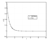
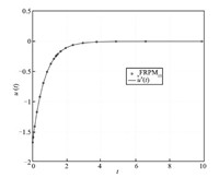
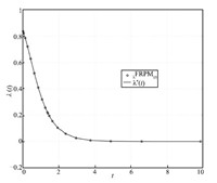
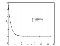
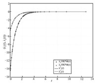
typical state,control,and costate solution for $N$ $=$ $20$ FLGR
points is shown in Figs. 1-3,respectively,along with the exact
solution. As can be seen,the FRPM solution agrees well with the
exact solution.
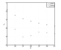
The maximum absolute errors between the FRPM solution and the exact
solution for Example 1 are defined as
|
\begin{array}{l}
e_x:=\max\limits_{i\in[0,N]}\log_{10}|x_i-x^*(t_i)|,
\end{array}
|
(58a)
|
|
\begin{array}{l}
e_u:=\max\limits_{i\in[1,N]}\log_{10}|u_i-u^*(t_i)|,
\end{array}
|
(58b)
|
|
\begin{array}{l}
e_\lambda:=\max\limits_{i\in[0,N]}\log_{10}|\lambda_i-\lambda^*(t_i)|.
\end{array}
|
(58c)
|
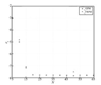
The maximum absolute errors of the state,the control,and the
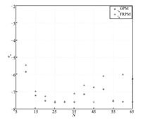
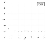
costate obtained using the GPM and FRPM are shown in Figs. 4-6,
respectively. The GPM is chosen as a baseline for comparison because
it results in a perfect match between the discretized optimality conditions and the KKT conditions,
and therefore,generates extremely accurate costate. It is seen that
$e_x$,$e_u$,and $e_\lambda$ decrease in a linear manner from $N=5$
to 20,demonstrating a spectral convergence rate for both of the
methods. Furthermore,all three errors remain essentially constant
for $N\geq30$.
B. Example 2: Infinite-horizon Linear Quadratic Regulator Problem
Consider the following infinite-horizon linear quadratic regulator
(LQR) problem[6, 12]. Determine the state,${\pmb x}(t)=$
$[x_1(t),x_2(t)]^{\rm T}R^2$,and the control,$u(t)\in
R$,on $t\in [0$,$+\infty)$ that minimize the cost functional
|
\begin{equation}
J=\frac{1}{2}\int_0^\infty\left({\pmb x}^{\rm T}{ Q}{\pmb x}+u^{\rm T}Ru\right)\rm{d} t,
\end{equation}
|
(59)
|
subject to the dynamic constraints
|
\begin{equation}
\dot{{\pmb x}}={ A}{\pmb x}+{\pmb B}u,
\end{equation}
|
(60)
|
and the boundary conditions
|
\begin{equation}
{\pmb x}(0)=\begin{bmatrix}
-4
4
\end{bmatrix},
\end{equation}
|
(61)
|
where
|
\begin{equation}
{ A}=\begin{bmatrix}
0 &1 \\
2 &-1
\end{bmatrix},\ {\pmb B}=\begin{bmatrix}
0 \\
1
\end{bmatrix},\ { Q}=\begin{bmatrix}
2 &0 \\
0 &1
\end{bmatrix},\ R=\frac{1}{2}.
\end{equation}
|
(62)
|
The exact solution to this problem is
|
\begin{array}{l}
{\pmb x}^*(t)=\exp([{ A}-{\pmb {BK}}]t){\pmb x}(0),
\end{array}
|
(63a)
|
|
\begin{array}{l}
u^*(t)=-{\pmb K}{\pmb x}^*(t),
\end{array}
|
(63b)
|
|
\begin{array}{l}
{\pmb \lambda}^*(t)={ S}{\pmb x}^*(t),
\end{array}
|
(63c)
|
where
|
\begin{array}{l}
{\pmb K} =\begin{bmatrix}
4.828427124746193 &2.557647291327851
\end{bmatrix},
\end{array}
|
(64a)
|
|
\begin{array}{l}
{S} =\begin{bmatrix}
6.031273049535752 &2.414213562373097
2.414213562373097 &1.278823645663925
\end{bmatrix}.
\end{array}
|
(64b)
|
In a manner similar to Example 1,the variable transformation
function $t=\zeta_c(\tau)$ was chosen to convert the LQR problem to
a finite-horizon problem,which was then solved using the FRPM with
the NLP solver SNOPT[15] for $N=40$. The optimality and
feasibility tolerances for the SNOPT were set to $10^{-6}$ and
$2\times10^{-6}$,respectively. The state,control,and costate are
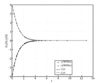
shown in Figs. 7-9,respectively,along with the exact solution. It
can be seen that the FRPM solution is virtually indistinguishable
from the exact solution.
The maximum absolute errors between the FRPM solution and the exact
solution for Example 2 are defined as
|
\begin{array}{l}
e_{{\pmb x}}:=\max_{i\in[0,N]}\log_{10}|{\pmb x}_i-{\pmb
x}^*(t_i)|,
\end{array}
|
(65a)
|
|
\begin{array}{l}
e_u:=\max_{i\in[1,N]}\log_{10}|u_i-u^*(t_i)|,
\end{array}
|
(65b)
|
|
\begin{array}{l}
e_{{\pmb \lambda}}:=\max_{i\in[0,N]}\log_{10}|{\pmb \lambda}_i-{\pmb
\lambda}^*(t_i)|.
\end{array}
|
(65c)
|
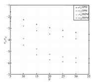
The maximum absolute errors of the state,the control,and the
costate obtained using the GPM and FRPM for $N=5$ to 35 are shown in
Figs. 10-12,respectively. It is seen that $e_{\pmb x}$,
$e_u$,and $e_{\pmb \lambda}$ decrease in a linear manner from
$N=5$ to 25,demonstrating a spectral convergence rate for the FRPM.
Furthermore,all three errors obtained using the FRPM remain
essentially constant for $N\geq25$. Finally,it is observed that the
GPM converges more slower than the FRPM in this example with the
magnitude of the errors being approximately two order larger.
Ⅵ. CONCLUSION
In this paper,a pseudospectral method has been presented for the
numerical solution of nonlinear infinite-horizon optimal
control problems using global collocation at flipped
Legendre-Gauss-Radau points. A new general change of variables is
proposed to convert the infinite-horizon problem into a
finite-horizon problem,which is then solved by FRPM. This general
transformation maps the scaled left half-open interval $\tau$ $\in$
$(-1,$ $+1]$ to the descending time interval $t\in(+\infty,0]$,and
thus,the singularity of collocation at point $+1$ associated with
the commonly used transformation is avoided. The costate and
constraint multiplier estimates for the FRPM are rigorously derived
by comparing the discretized necessary optimality conditions of a
finite-horizon problem with the Karush-Kuhn-Tucker conditions of the
resulting nonlinear programming problem from collocation. The method
has been applied to two infinite-horizon optimal control problems
taken from the open literature,and the numerical results indicate
that it leads to the ability to determine accurate solutions on the
entire horizon including $t=+\infty$. Other pseudospectral methods,
particulary the Gauss pseudospectral method,for solving
infinite-horizon optimal control problems with the proposed
transformation should be investigated for future work.

 2016, Vol.3


