I. INTRODUCTION

As is well known, adaptive control is an effective method in dealing with parameter uncertainties of a system^{[1, 2]}. Most results of adaptive control only provide boundedness and asymptotic performance of signals. Large transient error may arise in the beginning of a control process. In practical control, however, the boundedness and asymptotic performance is far from being enough to determine the feasibility of a system. Both the steady-state response and the transient response should be taken into account simultaneously in order to control a system successfully.

For this reason, much effort has been made to improve the transient performance of adaptive control^{[3, 4, 5]}. The most widely known method is the multiple model adaptive control (MMAC) method in which a family of candidate controllers and a supervisor are designed^{[6, 7, 8]}. The estimators of candidate controllers have different initial values that are evenly distributed over the range of uncertainty, and the supervisor selects the controller whose corresponding estimator has the smallest estimation error. The essence of this method is to ensure that the estimation error is small all the time. As a result, a better transient response comes at the cost of complexity. Simulations have shown the superiority of MMAC over conventional adaptive control, while some basic performance indices, such as the overshoot and rise time, still remain unclear.

An exponential convergence rate exists for linear adaptive control systems when the input signal is persistently exciting^{[9, 10]}. In the absence of persistently exciting input signal, however, it is difficult to guarantee any transient bound in adaptive control due to the unknown parameters. In order to characterize the transient behavior of adaptive control more precisely, in recent years, researchers have devoted their efforts to find a decaying bound for the transient period. A few preliminary results have been reported. In ^[11], the tracking error is contained in a prescribed performance funnel with no asymptotical tracking obtained. By means of transforming the constrained problem into a boundedness problem, asymptotical tracking with a prescribed performance is achieved for strict feedback systems (see ^{[12, 13, 14]} and the references therein). The strict feedback structure, however, is very special, which limits the application of this method. For a more general system structure in adaptive control, a switching strategy is proposed in ^[15] to guarantee a transient bound by selecting the right parameter value within a discrete finite set.

Both in MMAC and the approach of ^[15], switching plays an important role in enhancing control performance. In fact, the idea of using switching to improve the performance of adaptive control can be traced back to ^[16]. The switched controllers make the closed loop adaptive control system a switched system which has been widely studied in recent decades. A switched system is composed of a switching law and a family of subsystems that share a common state. Through splicing the dynamics of different subsystems, the switching signal endows the switched system with properties that its subsystems do not possess. Plenty of analyzing and designing methods have been reported for switched systems^{[17, 18, 19, 20, 21]}.

On the other hand, reset control is another approach to improve transient behavior and is drawing growing attention in recent years^{[22, 23]}. Reset controllers are dynamic controllers with reset states. In a way, the reset controller extracts energy from the system and then cut off the energy away by resetting. Thus, a properly designed reset principle can speed up the convergence rate of the control system. Typically, the reset mechanism can overcome the wind-up problem of the integral controller and reduce the overshoot dramatically^{[24, 25]}. Some preliminary methods on how to design reset principle and guarantee stability have been presented^{[26, 27, 28, 29]}. Unlike the switched system, the discontinuity of energy is the essence of reset control in enhancing the control performance. With one fixed control law, however, the reset controller cannot obtain new properties as a switched system does. Therefore, we are hopeful to further improve the transient performance of adaptive control via combining the ideas of switching and resetting.

What makes the transient behavior elusive in direct adaptive control~ (indirect adaptive control)\hfill is the interaction between the control error (state estimation error, respectively) and the parameter estimation error. It is generally accepted that a large parameter estimation error tends to increase the control error (state estimation error). On the other hand, the control error (state estimation error) also affects the estimation process. The integral term in an adaptive law is always adjusting the estimate while the control error (state estimation error) is not zero. Therefore, when the control error (state estimation error) is large, the estimate changes fast no matter how small the estimation error is. As a result, the estimate could be driven away far from its ideal value, which is called over-adaptation in ^{[30, 31]}, and this deflected estimate of the unknown parameter, in turn, is likely to arouse a growth of the control error (state estimation error). This is why a good initial estimate often ends up with bad transient performance. The over-adaptation is weakened by the methods provided in ^{[30, 31]} from the standpoint of application, but it is still an open problem on how to avoid over-adaptation mechanically.

To alleviate the effect of control error on adaptation, some information of the unknown parameter is helpful in modifying the adaptive law. For instance, the bound of the uncertainty parameter is used to construct a so called projection adaptive law^{[32, 33]}. The projection mechanism prevents the estimate from going outside the scope of the unknown parameter and thus achieves a better transient response. It is natural to expect a better control performance with more specific information about the unknown parameter.

One can get a pretty accurate value of the unknown parameter by identifying it beforehand. Numerous methods have been provided to identify the uncertain parameter of a system. Usually, the estimate converges to the real parameter value asymptotically or exponentially, which means that we cannot obtain the accurate estimate within finite time. It is recently claimed in ^[34] that the real value of the unknown parameter can be calculated within finite time. However, in the presence of disturbances, this identification is also inaccurate. As is discussed above, using this pre-estimate as the initial estimate in adaptive control cannot guarantee a good transient performance although it is pretty close to the real value. If we use this inaccurate pre-estimate without adaptation, asymptotical property would be lost. Inaccurate as the pre-estimate is, it could be helpful in amending the adaptive law, for instance, to reset the parameter estimate. To the best of our knowledge, no results on reset adaptive control are reported in the published literature.

In this paper, with the pre-estimation given, the resetting and switching strategies are developed for the adaptive control law so that certain transient performance is ensured for the closed-loop nonlinear adaptive control system. When it comes to the linear system, exponential decaying rate is ensured by the proposed method. Both the ideas of supervisory control and Lyapunov-like functions are applied in the designing process. The result has three features. Firstly, reset mechanism is involved in adaptive law to ensure the decaying rate. Secondly, for a class of uncertain nonlinear systems, a transient performance is ensured for adaptive control. Finally, the proposed reset adaptive law differs form the projection adaptive law in a way that the parameter estimation error may go beyond its bound even if the bound is known, for the over adaptation could be helpful in some specific conditions and should not be prohibited.

The structure of the paper is as follows. In Section II, we formulate the problem and present some preliminaries. The switched reset adaptive law is presented in Section III. Simulation is given in Section IV. Section V gives the conclusions and future directions of the research.

${\bf Notations}$. Throughout the paper, ${\bf R}^X$ denotes the $X$-dimension real space, $\lambda_{\rm min}(\cdot)$ denotes the minimum eigenvalue of a matrix, $\lambda_{\rm max}(\cdot)$ denotes the maximum eigenvalue of a matrix, $\|\cdot\|$ denotes the Euclidean norm of a vector, $|\cdot|$ denotes the absolute value of a scalar.

II. PROBLEM FORMULATION AND PRELIMINARIES

A. Problem Formulation and Assumptions

Adaptive control considers systems containing unknown parameters^{[1, 2, 10, 32]}

\begin{align} \dot x = \mathbb{f}(x, \theta^*, u), \end{align}

(1)

where $x \in {{\bf R}^n}$ and $u$ are the system state and the control input, $\theta ^*\in{{\bf R}^m}$ is the constant unknown parameter vector. Normally, it is demanded that $\theta^*$ is a linear parameter in $\mathbb{f}$. An estimation $\hat \theta$ is used instead of $\theta^*$ in the feedback control law $u=g(x, \hat \theta)$ according to the certainty-equivalence principle. Thus, an error system is derived with the parameter estimation error contained in the input, and the error system is stable when the estimation error is zero.

From this view point, we directly consider the following nonlinear system

\begin{align} \dot x = f(x) + g(x)\Phi (t)(\hat \theta - \theta ^*), \end{align}

(2)

where $\Phi :[0, \infty ) \to {{\bf R}^{1 \times m}}$ is a known bounded continuous function with $\| {\Phi ( \cdot )} \| \le M$ for some positive constant $M, f(x):{{\bf R}^{n}}\to {{\bf R}^{n}}$ and $g(x):{{\bf R}^{n}}\to {{\bf R}^{n}}$ are known locally Lipschitz functions satisfying $f(0) = 0$.

The control objective is twofold. Design a switched reset adaptive law for the estimate $\hat \theta $ in system (2) such that

1) all signals of the closed-loop system are bounded and the system state $x$ converges to zero, i.e., $\mathop {\lim }\nolimits_{t \to \infty } x(t) = 0$;

2) for a given pre-estimate $\bar \theta $ with $\| {\bar \theta - {\theta ^*}}\| \le d, d$ being a constant, a transient boundary is ensured for $x$.

${\bf Remark 1.}$ In traditional adaptive control, to cope with the　uncertainties, adaptive law is designed for the estimation parameter $\hat \theta$ so that the first objective can be achieved. Here, we concentrate on how to achieve the second objective via resetting the estimation parameter.

${\bf Remark 2.}$ The pre-estimate $\bar \theta$ and $d$ are assumed to be given beforehand. If the unknown parameter belongs to a known compact set $\Omega$, intuitively, we can choose the center of $\Omega$ as $\bar \theta$ in order to minimize $d$. Otherwise, we can calculate the pre-estimate within finite time using the method proposed in ^[34].

${\bf Remark 3.}$ Actually, $\Phi ( \cdot )$ is often a function of several arguments subject to time $t$. Because the bounds of these arguments usually rely on $x$, all we need is that the continuity of $\Phi$ with respect to its arguments if the bound of $x$ is known.

${\bf Definition 1.}$^[35] A continuous function $\alpha : [0, a) \to [0, \infty)$ is said to belong to class ${\mathcal {K}}$ if it is strictly increasing and $\alpha(0)=0$. It is said to belong to class ${\mathcal {{K}_\infty}}$ if $a=\infty $ and $\alpha (r)$ $\to\infty$ as $r\to \infty$.

${\bf Definition 2.}$^[35] A continuous function $\beta :[0, a)\times [0, \infty )\to[0, \infty )$ is said to belong to class ${\mathcal {KL}}$ if, for each fixed $s$, the mapping $\beta(r, s)$ belongs to class ${\mathcal {K}}$ with respect to $r$ and, for each fixed $r$, the mapping $\beta(r, s)$ is decreasing with respect to $s$ and $\beta(r, s)\to 0$ as $s\to \infty$.

The result of this paper is based on the following assumption.

${\bf Assumption 1.}$ There exist positive definite functions ${V_1}(x), G(x)\in{C^1}$ and class ${\mathcal {{K}_\infty} }$ functions ${\alpha _1}( \cdot )$ and ${\alpha _2}( \cdot )$, such that for all $x \in {{\bf R}^n}$,

\[\frac{{\partial {V_1}}}{{\partial x}}f(x) = - G(x), \]

(3)

\[{\alpha _1}(\left\| x \right\|) \le {V_1}(x) \le {\alpha _2}(\left\| x \right\|).\]

(4)

It is also assumed that there exists a $r>0$ so that

\begin{align} G(x)> lMd\left|\frac{{\partial {V_1}}}{{\partial x}}g(x)\right| \end{align}

(5)

holds for all $\|x\|>r$, where $l>1$.

${\bf Remark 4.}$ Equation (5) is to ensure that $f(x)$ plays a dominating role in the time derivative of $V_1$ along system (2).

${\bf Remark 5.}$ A special case of (5) is

\begin{align} \mathop {\lim }\limits_{x \to \infty } \frac{{\frac{\partial{V_1}}{\partial x} {g(x)}}}{G(x)} = 0. \end{align}

(6)

The condition (3) ensures that we can always find a $V_1$ satisfying (6) for a linear system

\begin{align} \dot x = Ax + B\Phi (t)(\hat \theta - {\theta ^*}), \end{align}

(7)

where $A\in {\bf R}^{n\times n}, B\in {\bf R}^{n}$. Equation (3) means that the autonomous system of (7), i.e.,

\begin{align} \dot x = Ax \end{align}

(8)

is asymptotically stable. Hence, there exist positive definite matrices $P$ and $Q$ satisfying^[36]

\[{A^{\rm{T}}}P + PA = - Q.\]

(9)

Choosing ${V_1}(x) = {x^{\rm T}}Px, G(x) = {x^{\rm T}}Qx$ and using the fact that $g(x) = B$ lead to

\begin{align} \frac{\frac{\partial {{V}_{1}}}{\partial x}g(x)}{G(x)} & =\frac{2{{x}^{\rm T}}PB}{{{x}^{\rm T}}Qx} \notag\\[1mm] & \le \frac{2\left\| {{x}^{\rm T}}PB \right\|}{\left\| {{x}^{\rm T}}Qx \right\|} \notag\\[1mm] & \le \frac{2\left\| x \right\|\left\| PB \right\|}{{{\lambda }_{\rm min}}(Q){{\left\| x \right\|}^{2}}}, \end{align}

(10)

which satisfies (6).

B. Motivation

In order to state our motivation, we first recall the basic idea of traditional adaptive control. Normally, a positive definite function is chosen as the Lyapunov function in the Lyapunov-based design method^[1]

\begin{align} V = {V_1} + \frac{1}{2\gamma}{{\tilde \theta }^{\rm T}}\tilde \theta, \end{align}

(11)

where $\tilde \theta = \hat \theta - {\theta ^*}$ is the estimation error, $\gamma $ is a positive number.

Taking the time derivative of (11) into account gives

\begin{align} \dot{V}={{\dot{V}}_{1}}+\frac{1}{2\gamma }{{\tilde{\theta }}^{\rm T}}\tilde{\theta }=\frac{\partial {{V}_{1}}}{\partial x}\dot{x}+\frac{1}{\gamma }{{\tilde{\theta }}^{\rm T}}\dot{\tilde{\theta }}. \end{align}

(12)

Using (2), we know

\begin{align} \dot{V}& ={{{\dot{V}}}_{1}}+\frac{1}{2\gamma }{{{\tilde{\theta }}}^{\rm T}}\tilde{\theta }\notag\\[1mm] & =\frac{\partial {{V}_{1}}}{\partial x}\left( f(x)+g(x)\Phi \tilde{\theta } \right)+\frac{1}{\gamma }{{{\tilde{\theta }}}^{\rm T}}\dot{\tilde{\theta }} \notag\\[1mm] & =\frac{\partial {{V}_{1}}}{\partial x}f(x)+\frac{\partial {{V}_{1}}}{\partial x}g(x)\Phi \tilde{\theta }+\frac{1}{\gamma }{{{\tilde{\theta }}}^{\rm T}}\dot{\tilde{\theta }} \notag\\[1mm] & =\frac{\partial {{V}_{1}}}{\partial x}f(x)+{{{\tilde{\theta }}}^{\rm T}}{{\Phi }^{T}}{{g}^{\rm T}} (x){{\left( \frac{\partial {{V}_{1}}}{\partial x} \right)}^{\rm T}}+\frac{1}{\gamma } {{{\tilde{\theta }}}^{\rm T}}\dot{\tilde{\theta }}. \end{align}

(13)

So, the following adaptive law

\begin{align} \dot {\tilde \theta} = \gamma {\Phi ^{\rm T}}{g^{\rm T}}(x){\left( {\frac{{\partial {V_1}}}{{\partial x}}} \right)^{\rm T}}, \end{align}

(14)

and (3) ensure that the time derivative of $V$ along system (2) is

\begin{align} \dot V = - G(x), \end{align}

(15)

which leads to signal boundedness and state convergence of system (2).

Since $V$ is composed of both $x$ and $\tilde \theta$, the decrease of $V$ do not indicate the decrease of $\| x \|$. When the initial value of $\tilde \theta $ is large, $\| x \|$ could become extremely large even if the initial state $\| {x({t_0})} \|$ is zero. This is why one wants to make the initial value of $\hat \theta $ close to $\theta^*$. Conversely, a large initial tracking error can also cause a tremendous growth of $\tilde \theta $, which means that a large estimation error could appear even if the estimate is accurate at the beginning. Therefore, a good initial estimate does not always lead to a good control performance. Now, using an example, we show the drawback of the integral adaptive law.

Consider the state tracking problem of a linear system

\begin{align} \dot x = x + u, ~~x(0) = 1. \end{align}

(16)

The desired state trajectory $x_m$ is generated by

\begin{align} \dot x_m =-x_m + v, ~~x_m(0) = 0. \end{align}

(17)

Now we design an adaptive controller for (16) such that the tracking error $e = {x_m} - x$ converges to zero, i.e., $\mathop {\lim }\nolimits_{t \to \infty } e(t)=0$.

Subtracting (16) from (17) and using the controller

\begin{align} u = \hat \theta x + v, \end{align}

(18)

we obtain the dynamics of the tracking error

\begin{align} \dot e = - e + ( - \hat \theta - 2)x=-e-\tilde \theta x. \end{align}

(19)

The tracking problem comes down to a convergence problem of the error system (19) which is of form (2). Choose a candidate Lyapunov function

\begin{align} V = \frac{1}{2}{e^2} + \frac{1}{2}{\tilde \theta ^2}. \end{align}

(20)

The adaptive law

\begin{align} \dot{\hat \theta } = ex \end{align}

(21)

leads to

\begin{align} \dot V = - {e^2}, \end{align}

(22)

which ensures $\mathop {\lim }\nolimits_{t \to \infty } e(t) = 0$.

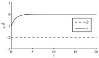
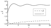
Obviously, the ideal value of $\hat \theta$ is $-2$. Suppose we have a pre-estimated value $-1.99$ for $\theta^*$. We first use a constant estimate with $\hat \theta \equiv - 1.99$ and then we use the adaptive estimation (21) with $\hat \theta (0) = - 1.99$ in the simulation. The simulation results in Figs. 1 and 2 show that the controller with the constant estimation has a better transient performance in spite of the steady state error. The controller with the adaptive estimation, although can ensure asymptotical tracking, causes oscillations in the transient period. This is because, due to the presence of a large initial error, the adaptive law (21) drives the estimate $\hat \theta $ far away from its ideal value $-2$, and the deflected estimate in the controller, in turn, causes an increase of the tracking error $e$. Thus, just like the wind up problem of integral control, oscillations emerge due to the blindness of adaptation. The constant estimation, of course, does not have this problem.

The first thought is that a proper switching between the non-adaptive controller and the adaptive controller can achieve both good transient performance and asymptotical tracking. More specifically, it is advisable to use the non-adaptive controller while the tracking error is large and switch to the adaptive controller when the tracking error is small enough.

A further consideration of the large error period suggests that turning off the adaptation is not necessary in order to maintain the good transient performance. An adaptive controller could behave better than the non-adaptive one if the estimation does not deviate seriously. Hence, the key problem is how to avoid over-adaptation. Intuitively, if the adaptive controller is doing worse than the non-adaptive one, we have a reason to reset the estimate in the adaptive controller with the value of the pre-estimate.

Thus, here come the problems of where to switch and when to reset, which we are going to discuss in the following section.

III. SWITCHED RESET ADAPTIVE LAW

This section discusses how to improve the transient performance of system (2) while preserving the asymptotical convergence property by using the switched reset adaptive law. We state our result in three parts. First, the pre-estimated value is used for system (2) without adaptation and the transient performance is analyzed. Then, a switched reset adaptive law is proposed by introducing a supervisory variable to achieve both transient bound and asymptotical convergence. Further, we replace Assumption 1 with Assumption 2 in order to obtain an exponentially decaying bound of $x$, which ensures that the state $x$ can reach a definite ball within a finite time and remain inside thereafter.

A. Constant Estimation

It follows from Assumption 1 that

\begin{align} \frac{G(x)}{l}> Md\left|\frac{{\partial {V_1}}}{{\partial x}}g(x)\right|, \quad x \in {{\bf R}^n}\backslash {B_{r}}, \end{align}

(23)

where $B_{r}=\left\{x|\left\|x\right\|\le r\right\}$.

Let $\partial B_{r}=\{x|\left\|x\right\|=r\}$ be the boundary of the ball $B_{r}$ and let $t_{k_-}$ and $t_{k_+}$ ($k=1, 2, \ldots $) denote the time instants when $x$ reaches $\partial B_{r}$ from outside and inside respectively.

Construct a $\mu$-system

\begin{align} \begin{cases} \dot \mu = - \epsilon{S_{{V_1}}}(\mu ), & t \ne {t_{{k_ + }}}, \\[1mm] \mu ({t_{{k_ + }}}) = (1 + \delta ){V_1}({t_{{k_ + }}}), & t = {t_{{k_ + }}}, \end{cases} \end{align}

(24)

with $\mu ({t_0}) > {V_1}(x(t_0))$, where $\delta$ is a small positive number, $0<\epsilon<1$ and ${S_{{V_1}}}( \cdot )$ is some positive definite function to be chosen later.

A special version of~(24) without resetting was used in ^[15]. Using the positive definiteness of ${S_{{V_1}}}( \cdot )$ and applying the Lemma 4.4 in ^[35] give

\begin{align} \begin{cases} \mu (t) = \beta (\mu ({t_0}), t - {t_0}), & {t_0} \le t \le {t_{{1_ + }}}, \\[1mm] \mu (t) = \beta (\mu ({t_{{k_ + }}}), t - {t_{{k_ + }}}), & {t_{{k_ + }}} \le t \le {t_{{{(k + 1)}_ + }}}, \end{cases} \end{align}

(25)

where $\beta$ is a class $\mathcal{KL}$ function.

${\bf Theorem 1.}$ When a constant estimate $\hat \theta \equiv \bar \theta $ with $\|\bar \theta$ - $\theta^*\|\le d$ is used for system (2), $\| x \|$ is bounded by $\alpha _1^{ - 1}(\mu )$ outside the ball ${B_{r}}$. Moreover, if $x(t_0)$ is outside a ball ${B_{r'}}=\left\{ {x| {\left\| x \right\| \le r'=\alpha _1^{ - 1}\circ{\alpha _2}(r)} } \right\}$, then, $x$ reaches the ball $B_{r'}$ within a finite time $T$ and remains inside for all $t\ge T$.

${\bf Proof.}$ Since $\|\Phi(t)\|\le M$ and $\|\hat \theta-\theta^*\|=\|\bar \theta-\theta^*\|\le d$, the time derivative of $V_1$ along (2) satisfies

\begin{align} {{\dot V}_1}& = \frac{{\partial {V_1}}}{{\partial x}}f(x) + \frac{{\partial {V_1}}}{{\partial x}}g(x)\Phi(t) \left( {\hat \theta - {\theta ^*}} \right)\notag\\[1mm] &\le - G(x) + \left| {\frac{{\partial {V_1}}}{{\partial x}}g(x)} \right|Md. \end{align}

(26)

Noticing (23), we have

\begin{align} {{\dot V}_1}< - (1-\frac{1}{l}){G(x)}= - S(x), \quad x \in {{\bf R}^n}\backslash {B_{r}}. \end{align}

(27)

Because $S( \cdot )$ is continuous and positive definite and ${V_1}$ is radially unbounded, one can find a positive definite function ${S_{{V_1}}}( \cdot )$ such that

\begin{align} {\dot V_1} < - S(x)= - {S_{{V_1}}}({V_1}) \end{align}

(28)

for all $x \in {{\bf{R}}^n}\backslash {B_r}$^[15].

Without loss of generality, we assume $\|x_0\|>r$. Noticing (24), (28) and applying the comparison theory to the time intervals $[t_0, t_{1_-}), [t_{k_+}, t_{(k+1)_-})$, for all $x \in {\bf R}^n\backslash {B_{r}}$, we obtain

\begin{align} {V_1}(x(t)) < \mu (t). \end{align}

(29)

By (4) and (29), we know that

\begin{align} \left\| {x(t)} \right\| \le \alpha _1^{ - 1}({V_1}(x(t))) < \alpha _1^{ - 1}(\mu ), ~~ x\in {\bf R}^n \backslash B_{r}. \end{align}

(30)

Now, we show the existence of the ball $B_{r'}$.

To this end, we first prove that, if $x(t_0)\notin B_{r'}, x$ reaches the ball $B_{r}$ within a finite time. If this is not true, i.e., $t_{1_{-}}=\infty$, then, (4) implies $V_1(x(t))\ge \alpha_1(\|x(t)\|) \ge \alpha_1(r)$. Since $\beta$ is a class $\mathcal {KL}$ function, there exists a $T, {t_0} < T < \infty $ such that $\mu (t) = \beta (\mu ({t_0}), t - {t_0}) < {\alpha _1}(r)$ for all $t > T$. That is, we have $V_1(x(t))>\mu(t)$ for all $t > T$ and $x\notin {B_{r}}$, which conflicts with (29). Hence, $x$ reaches the ball $B_{r}$ within a finite time $T$ and, of course, $T \ge {t_{1\_}}$.

Although $x$ may pass across $\partial B_{r}$ repeatedly, we can still find another ball $B_{r'}$ that contains $x$ for all $t > {t_{1\_}}$. Actually, for all ${t_{{k_ + }}} \le t \le {t_{(k + 1)\_}}$ , using (27) and (4), we have

\begin{align} \left\| {x(t)} \right\| & \le \alpha _1^{ - 1}\left( {{V_1}\left( {x(t)} \right)} \right)\notag\\[1mm] & \le \alpha _1^{ - 1}\left( {{V_1}\left( {x({t_{{k_+ }}})} \right)} \right)\notag\\[1mm] & \le \alpha _1^{ - 1}\circ{\alpha _2}\left( {\| {x({t_{{k_+ }}})} \|} \right)\notag\\[1mm] & = \alpha _1^{ - 1}\circ{\alpha _2}( r )=r'. \end{align}

(31)

According to (4), $\alpha _1^{ - 1}\circ{\alpha _2}\left( r \right)\ge r$ holds, namely,

\begin{align} B_{r}\subseteq {B_{r'}} . \end{align}

(32)

So, $x$ reaches the ball $B_{r'}$ within the finite time $T$ and remains inside for all $t\ge T$.

$\square$

${\bf Remark 6.}$ Under Assumption 1, $\dot V_1<\dot \mu$ is ensured by $\|\tilde \theta\|\le d$ outside the ball $B_{r}$. Given $x(t_0) \notin B_{r}$ and $V_1(t_0)<\mu(t_0)$, we have $V_1<\mu$ before $x$ goes into the ball $B_{r}$. Although $V_1$ may surpass $\mu$ while $x$ is inside the ball $B_{r}$, the reset of $\mu$ at time $t_{k_+}$ ensures that $V_1<\mu$ for all $\|x\|>r$.

${\bf Remark 7.}$ For all $\|x\|>r, V_1<\mu$ also holds for a non-constant estimate $\hat\theta$ if $\| {\hat \theta - {\theta ^*}} \| = \| {\tilde \theta } \| \le d$, which is easy to see from the proof of Theorem 1.

${\bf Remark 8.}$ If the pre-estimation is accurate, i.e., $d = 0$, asymptotical state convergence follows from (26). When $d > 0$, however, the convergence of $x$ cannot be obtained using constant estimation.

${\bf Remark 9.}$ When $V_1=\alpha(\left\|x\right\|)$ for some class $\mathcal{K_\infty}$ function $\alpha$, we have $\alpha_1(\cdot)=\alpha_2(\cdot)$ and thus $r'=\alpha _1^{ - 1}\circ{\alpha _2}(r)=r$, which means ${B_{r'}}={B_{r}}$. B. Switched Reset Adaptive Law

The constant estimate studied in Subsection III. A, although ensures a transient bound outside the ball ${B_{r}}$, cannot achieve asymptotical convergence. On the other hand, a non-constant estimate with adaptation mechanism can achieve asymptotical convergence with no transient bound guaranteed. Is it possible for an adaptive estimation to gain both transient bound and asymptotical convergence? This is what we are about to discuss in this subsection. In fact, an adaptive estimation has the same transient bound as the constant one if

\begin{align} \| {\hat \theta - {\theta ^*}} \| = \| {\tilde \theta } \| \le d \end{align}

(33)

is satisfied during the adaptation process. To achieve both asymptotical convergence and transient bound, we should amend the adaptive law using $\bar \theta $ to avoid some blindness in adaptation. More specifically, reset $\hat \theta $ with $\bar \theta $ when $\| {\tilde \theta } \| > d$. Since ${\theta ^*}$ is unknown, it is not an easy task to identify the moment when $\| {\tilde \theta } \|$ exceeds the limit $d$. Based on the proof of Theorem 1, for all $x\notin {B_{r}} $, we have $V_1<\mu$ if $\| \hat \theta$ - ${\theta ^*} \|=\| {\tilde \theta } \| \le d$. In other words, outside the ball ${B_{r}}$, $V_1<\mu$ is violated only if $\| {\tilde \theta } \| > d$. If there are moments greater than $t_0$, for simplicity, let ${t^*}$ be one such a moment, at which ${V_1}(x({t^*}))=\mu({t^*})$ and $\|x({t^*})\|>r$, we have $\| {\tilde \theta ({t^*_-})} \|>d$. Therefore, it is reasonable to reset $\hat \theta $ with the pre-estimate $\bar \theta $ whenever ${V_1}(x({t})) = \mu({t})$ outside the ball $B_{r}$. Thus, we can employ $\mu$ as a supervisory variable to dominate the resetting of $\hat \theta $.

This $\mu$-supervised resetting is effective only when $x$ is outside the ball ${B_{r}}$. So, we need to switch back to the conventional adaptation once $x$ goes into the ball ${B_{r}}$.

As a result, we get a switched reset adaptive law

\begin{align} \begin{cases} \dot {\hat \theta } = \gamma {\Phi^{\rm T}}{g^{\rm T}}(x){\left( {\dfrac{{\partial {V_1}}}{{\partial x}}} \right)^{\rm T}}, & {V_1} < \mu ~{\rm or}~ x \in {B_{r}}, \\[1mm] \hat \theta = \bar \theta , & {\rm otherwise}. \end{cases} \end{align}

(34)

${\bf Remark 10.}$ The logic based adaptive law (35) is actually a switched one that is composed of two adaptive laws. One is the supervised reset adaptive law outside the ball ${B_{r}}$ and the other is the traditional adaptive law inside the ball ${B_{r}}$. The switching surface is the boundary of the ball ${B_{r}}$. An equivalent expression of (34) is

\begin{align} \begin{cases} \dot {\hat \theta} = \gamma {\Phi ^{\rm T}}{g^{\rm T}}(x){\left( {\dfrac{{\partial {V_1}}} {{\partial x}}} \right)^{\rm T}}, & x \in {B_{r}}, \\[3mm] \begin{cases} \dot {\hat \theta} = \gamma {\Phi ^{\rm T}}{g^{\rm T}}(x){{\left( {\dfrac{{\partial {V_1}}} {{\partial x}}} \right)}^{\rm T}}, & {V_1} < \mu , \\[1mm] \hat \theta = \bar \theta , & {\rm otherwise }, \end{cases}& x \notin {B_{r}}. \end{cases} \end{align}

(35)

${\bf Theorem 2.}$ For the given pre-estimate $\bar \theta $, the switched reset adaptive law (34), when applied to system~(2), ensures that

1) Boundedness of all signals and state convergence, i.e., $\mathop {\lim }\nolimits_{t \to \infty } x(t)=0$;

2) $\left\|x(t)\right\|$ is bounded by a decaying signal $\alpha _1^{ - 1}(\mu (t))$ outside the ball ${B_{r}}$.

${\bf Proof.}$ We first prove 1).

Consider the positive definite function $V=V_1+\frac{1}{2\gamma}\tilde \theta^{\rm T}\tilde \theta$ given in (11).

During the continuous time intervals when no reset occurs, derivative of $V$ along system (2) and adaptive law (34) is

\begin{align} \dot V = - G(x) < 0, \quad \forall x \ne 0. \end{align}

(36)

At the reset time $t^*$, the reset mechanism in (34) ensures that $\| {\tilde \theta ({t^*_- })} \| >d \ge \| {\bar \theta } -\theta^*\| =\| {\hat \theta({t^*_+}) } -\theta^*\|= \| {\tilde \theta ({t^*_+})}\|$. Therefore,

\begin{align} V(x({t^*_-}))& = {V_1}(x({t^*_-})) + {\| {\tilde \theta ({t^*_-})}\|^2}\notag\\[1mm] & > {V_1}(x({t^*_+})) + {\| {\tilde \theta ({t^*_+})}\|^2}\notag\\[1mm] & = V({x(t^*_+})). \end{align}

(37)

Equations (36) and (37) ensure that $V$ is decreasing with respect to time. Hence, $V(x(t)) \le V(x({t_0}))$, which means $x$ and $\tilde \theta $ are bounded. It follows from (2) that $\dot x$ is bounded, which implies that $x(t)$ is uniformly continuous on $t$. Since $G( x )$ is continuous on ${{\bf R}^n}$, the function $G( x )$ is uniformly continuous within the compact set $\{ x| \left\| {x(t)}\right \| \le \alpha _1^{ - 1}( V(x({t_0}), \tilde \theta ({t_0})))\}$. Therefore, $G( {x(t)} )$ is uniformly continuous with respect to $t$.

Integrating both sides of (36) and using (37) lead to

\begin{align} \int_{{t_0}}^t {G(x(\tau )){\rm d}\tau } = V(x({t_0})) - V(x(t)) \le V(x({t_0})). \end{align}

(38)

It follows from Barbalat lemma that $\mathop {\lim }\nolimits_{t \to \infty } G\left( {x(t)} \right) = 0$. Thus, $\mathop {\lim }\nolimits_{t \to \infty } x(t) = 0$ follows from the positive definiteness of $G(x(t))$.

Now, we prove 2).

From the construction of $\mu$, we know $V_1(t_0)<\mu(t_0)$. As soon as $V_1$ catches $\mu$ outside the ball $B_{r}$, namely, $V_1(t^*)=$ $\mu(t^*)$ and $\|x(t^*)\|>r$, the reset action in (34) makes $\tilde \theta ({t^*}) \le d$. Hence, Equations (27) and (28) in the proof of Theorem 1 hold at the time $t^*$. It follows from (24), (27) and (28) that $\dot \mu(t^*)-\dot V_1(t^*)\ge (1-\epsilon)S(x(t^*))>0 $. Since both $\dot \mu$ and $\dot V_1$ are continuous with respect to $t$ for all $t\ne t^*$, there exists a $\varepsilon > 0$ such that ${\dot V_1}(x(t)) < \dot \mu (t)$ for all $t \in [t^*, \:t^* + \varepsilon]$. Therefore, there is always an interval between two adjacent resettings and there is no chance that ${V_1} > \mu $ outside the ball ${B_{r}}$. That is

\begin{align} V_1\left(x(t)\right)\le \mu (t), \quad x\in {\bf R}^n \backslash {B_{r}}. \end{align}

(39)

Taking Assumption 1 into account, we have $\left\|x(t)\right\| \le \alpha _1^{ - 1}\left(V_1\left(x(t)\right)\right) \le \alpha _1^{ - 1}(\mu (t))$ for all $x\in {\bf R}^n \backslash {B_{r}}$.

$\square$

${\bf Remark 11.}$ The number of switching on the switching surface $\left\{x|\left\|x\right\|=r\right\}$ is finite. Because $\mathop {\lim }\nolimits_{t \to \infty } x(t) = 0$ guarantees that there exists a finite time $T_1>0$ such that, for all $t>T_1$, we have $\left\|x(t)\right\| < r$.

${\bf Remark 12.}$ The reset mechanism ensures that $V(x({t^*_-})) \ge V(x({t^*_+}))$, which means that the resetting extracts energy from the system. This explains why a switched reset adaptive law can achieve a better response.

${\bf Remark 13.}$ The transient boundary cannot be defined arbitrarily. The transient boundary of $x$ is deduced based on the fact that $V_1$ has a decay rate outside the ball $B_r$. Hence, the transient boundary is related with the Lyapunov function chosen in the design process.

C. Exponential Decaying Bound

A decaying bound of $x$ is given in the previous subsection outside the ball ${B_{r}}$. However, no decaying rate is guaranteed. In this subsection, we show how an exponential decaying bound is obtained with the following assumption.

${\bf Assumption 2.}$ There exist positive definite functions ${V_1}(x), G(x)\in{C^1}$ and positive constants $a, c_1, c_2$ and $c_3$, such that for all $x \in {\bf R}^n$,

\[\frac{{\partial {V_1}}}{{\partial x}}f(x) = - G(x), \]

(40)

\[{c_1}{\left\| x \right\|^a} \le {V_1}(x) \le {c_2}{\left\| x \right\|^a}, \]

(41)

\[{c_3}{\left\| x \right\|^a} \le G(x).\]

(42)

Also, there is a $r>0$ so that

\[G(x) > lMd\left| {\frac{{\partial {V_1}}}{{\partial x}}g(x)} \right|\]

(43)

holds for all $\|x\|>r$, where $l>1$.

${\bf Remark 14.}$ Equations (40) and (43) here are identical to (3) and (5) in Assumption 1. For the linear system (7), condition (40) means that we can find positive definite matrices $P, Q$ so that $A$ satisfies (9) and (10). Hence, we can choose positive functions ${V_1}(x) = {x^{\rm T}}Px$ and $G(x) = {x^{\rm T}}Qx$ so that

\begin{align} \begin{cases} {\lambda _{\min}(P)}{\left\| x \right\|^2} \le {V_1}(x) = {x^{\rm T}}Px \le {\lambda _{\max}(P)}{\left\| x \right\|^2}, \\[1mm] {\lambda _{\min}(Q)}{\left\| x \right\|^2} \le G(x) = {x^{\rm T}}Qx \le {\lambda _{\max}(Q)}{\left\| x \right\|^2}, \\[1mm] G(x)> lMd\left| {\frac{{\partial {V_1}}}{{\partial x}}B} \right|, ~{\rm for ~ all}~\left\| x \right\| > \dfrac{{2lMd\left\| {PB} \right\|}}{{{\lambda _{\rm min}(Q)}}} = {r}, \end{cases} \end{align}

(44)

which satisfies (41), (42) and (43).

Here, we still use $t_{k_-}$ and $t_{k_+}$ ($k=1, 2, \ldots $) to denote the time instants when $x$ reaches $\partial B_{r}$ from outside and inside respectively.

Reconstruct the $\mu$-system as

\begin{align} \begin{cases} \dot \mu = - \bar \lambda \mu, & t\ne t_{k_+}, \\[1mm] \mu({t_{k_+}}) =(1+\delta) {V_1}({t_{k_+}}), &t=t_{k_+}, \end{cases} \end{align}

(45)

with $\mu({t_0}) > {V_1}({t_0})$, where $\delta$ is a small positive number and $\bar \lambda $ is some positive constant to be designed later.

From (45), we have

\begin{align} \begin{cases} \mu(t) = \mu({t_0}){{{\rm e}}^{ - {\bar{ \bf\lambda }}({{t}} - {{{t}}_{\bf{0}}})}}, &{t_0} \le t \le {{t}_{{1_ + }}}, \\[1mm] \mu(t) = {\mu}({{t}_{{k_ + }}}){{{\rm e}}^{ - {\bar{\bf \lambda }}({\bf{t}} - {{{{t}}}_{{{{k}}_ + }}})}}, & {{t}_{{k_ + }}} \le t \le {{t}_{{{(k + 1)}_ + }}}. \end{cases} \end{align}

(46)

${\bf Theorem 3.}$ For the given pre-estimate $\bar \theta $, the switched reset adaptive law (34) with $\mu$ generated by (45), when applied to system (2), ensures

1) Boundedness of all signals and state convergence, i.e., $\mathop {\lim }\nolimits_{t \to \infty } x(t) = 0$;

2) $\|x(t)\|$ is bounded by $(\frac{\mu(t)}{c_1})^\frac{1}{a}$ outside the ball ${B_{r}}$;

3) If the initial state $x(t_0)$ is outside the ball ${B_{r'}} =\{ x|\|x\|\le{( {\frac{{{(1+\delta)c_2}}}{{{c_1}}}} )^{\frac{1}{a}}}{ r}=r'\}$, then $x$ decays exponentially into ${B_{r'}}$ within a finite time $T' = {t_0} + \frac{1}{{\bar \lambda }}\ln ( \mu ({t_0})(1+\delta )^{ - 1}c_2^{ - 1}r^{ - a} )$ and stays inside for all $t>T'$.

${\bf Proof.}$ We first prove that $V_1(x(t))\le\mu(t)$ outside the ball $B_{r}$, which is discussed in two cases.

${\bf Case 1.}$ $\| {\hat \theta - {\theta ^*}} \| =\|\tilde \theta\| \le d$.

The time derivative of $V_1$ along system~(2) satisfies

\begin{align} {\dot V_1} \le - G(x) + \left| {\frac{{\partial {V_1}}}{{\partial x}}g(x)} \right|Md. \end{align}

(47)

Taking (43) into account, for all $x \notin {B_{r}}$, we have

\begin{align} \frac{1}{l}G(x) \ge \left| {\frac{{\partial {V_1}}}{{\partial x}}g(x)} \right|Md. \end{align}

(48)

Equations (47) and (48) ensures

\begin{align} {\dot V_1} \le - \frac{l-1}{l}G(x)=- {c_4}G(x), \quad x \in {{\bf R}^n}\backslash {B_{r}}. \end{align}

(49)

Noticing (41) and (42), we obtain

\begin{align} {{\dot V}_1} & \le - {c_4}{c_3}{\left\| x \right\|^a}\notag\\[1mm] & \le - \frac{{{c_4}{c_3}}}{{{c_2}}}{V_1}\notag\\[1mm] & = - \lambda {V_1}, \quad x \in {{\bf R}^n}\backslash {B_{r}}. \end{align}

(50)

Choose $\bar \lambda, 0<\bar \lambda < \lambda$. It follows from (50), (45) and the comparison theory that

\begin{align} {V_1}(x(t)) < \mu(t) \end{align}

(51)

for all $x \in {{\bf R}^n}\backslash {B_{r}}$ and $t>t_0$.

${\bf Case 2.}$ No insurance of the condition $\|\tilde \theta\| \le d$. The adaptation process may drive $\hat \theta$ far away from $\theta^*$ so that $\| {\hat \theta - {\theta ^*}} \|> d$. Therefore, there may be moments greater than $t_0$ when ${V_1}(x(t)) = \mu({t})$. Let ${t^*}$ be one such a moment, i.e., ${V_1}(x(t^*)) = \mu({t^*})$, we can deduct from the discussion of Case 1 that $\| {\tilde \theta ({t^*_-})} \|> d$.

Because the reset mechanism in~(34) makes $\| {\tilde \theta ({t^*})} \| \le d$ at time $t^*, V_1$ cannot surpass $\mu$ outside the ball ${B_{r}}$, i.e.,

\begin{align} {V_1}(x(t)) \le \mu({t}), \quad x \in {{\bf R}^n}\backslash {B_{r}}. \end{align}

(52)

In both cases, we have ${V_1}(x(t)) \le u({t}), x \in {{\bf R}^n}\backslash {B_{r}}$. Therefore, Assumption 2 ensures

\begin{align} \|x(t)\| & \le {\left( {\frac{1}{{{c_1}}}{V_1}(x(t))} \right)^{\frac{1}{a}}}\notag\\[1mm] & \le {\left( {\frac{{\mu(t)}}{{{c_1}}}} \right)^{\frac{1}{a}}}, \quad x \in {{\bf R}^n}\backslash {B_{r}}. \end{align}

(53)

Using (53) and (46), for all $x(t_0) \in {{\bf R}^n}\backslash {B_{r'}}$ and $t\in [t_0, t_{1-})$, we have

\begin{align} \left\| {x(t)} \right\| \le {\left( {\frac{{\mu ({t_0})}}{{{c_1}}}} \right)^{\frac{1}{a}}}{{{\rm e}}^{ - \frac{{\bar \lambda }}{a}(t - {t_0})}}. \end{align}

(54)

Noticing $r'={( {\frac{{{(1+\delta)c_2}}}{{{c_1}}}})^{\frac{1}{a}}}{ r}$, we know that $x$ will reach the ball $B_{r'}$ within a finite time

\begin{align} T' = {t_0} + \frac{1}{{\bar \lambda }}\ln \left( {\mu ({t_0}){{(1 + \delta )}^{ - 1}}c_2^{ - 1}r^{ - a}} \right). \end{align}

(55)

Now, we turn to prove that $\|x\|\le{r'}$ for all $t>T'$. Equation (54) ensures $\|x\|$ keep decaying after $T'$ until $t_{1_-}$. From the definition of $t_{k_-}$ and $t_{k_+}$, we know that $\|x\|\le r \begin{align} \left\| {x(t)} \right\| & \le {\left( {\frac{{{(1+\delta)c_2}}}{{{c_1}}}} \right)^{\frac{1}{a}}}{{{\rm e}}^{ - \frac{{\bar \lambda }}{a}(t - {t_{{k_ + }}})}}\left\| {x({t_{{k_ + }}})} \right\|\notag\\[1mm] & \le {\left( {\frac{{{(1+\delta)c_2}}}{{{c_1}}}} \right)^{\frac{1}{a}}}\left\| {x({t_{{k_ + }}})} \right\|\notag\\[1mm] & = {\left( {\frac{{{(1+\delta)c_2}}}{{{c_1}}}} \right)^{\frac{1}{a}}}{r}=r'. \end{align} (56) Obviously, $x(t)$ remains inside $B_{r'}$ for all $t>T'$.

Finally, we prove 1). Since $\| {\tilde \theta ({t^*_-})} \| > d\ge \| {\tilde \theta ({t^*_+})} \| $, for the positive definite function $V = {V_1} + \frac{1}{2\gamma}{\| {\tilde \theta } \|^2}$ given by (11), the switched reset adaptive law (34) guarantees

\begin{align} \begin{cases} \dot V = - G(x) \le - {c_3}{\left\| x \right\|^a}, &t \ne {t^*}\\[1mm] V({t^*_ -}) \ge V({t^*_+}), & t = {t^*} \end{cases}. \end{align}

(57)

Similar to the proof of Theorem 2, (57) ensures the boundedness of $x, \tilde \theta$ and that $\mathop {\lim }\nolimits_{t \to \infty } x(t) = 0$.

$\square$

IV. SIMULATION

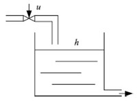
In this section, we illustrate the effectiveness of the proposed method using a water tank shown in Fig. 3. The dynamics of the water tank are

\begin{align*} \dot h = ku - \theta^* \sqrt h, \end{align*}

( )

where $h$ is the water level, $u$ is the opening of the inlet valve, $k$ is the coefficient of the inlet valve and $\theta^*$ is the unknown parameter. Our purpose is to regulate the water level $h$ to $h_r$.

Fig. 3

	Download: JPG larger image
Fig. 3 Water tank.

Define $e = h - {h_r}$ and let

\begin{align*}u = \frac{1}{k}\left( { - e + \hat \theta \sqrt h } \right).\end{align*}

( )

We have

\begin{align*} \dot e = - e + \left( {\hat \theta - \theta^* } \right)\sqrt h, \end{align*}

( )

which is a system of form (2). Suppose $\theta^* = 5$ and the pre-estimate is $\bar \theta = 4.95$, we run the simulation using the traditional adaptive law and the switched reset adaptive law respectively.

A. Traditional Adaptive Law

Choosing $V = \frac{1}{2}{e^2} + \frac{1}{{2\gamma }}{\tilde \theta ^2}$ leads to the adaptive law

\begin{align*} \dot {\hat \theta} = - \gamma e\sqrt h. \end{align*}

( )

We run the simulation with different $\gamma $ and the following parameters

\begin{align*} {h_r} = 10, \;\;h(0) = 0, \;\;\hat \theta (0) =\bar \theta= 4.95. \end{align*}

( )

The transient responses are shown in Fig. 4. Oscillations appear when $\gamma $ is large due to the over adaptation problem. One may argue that a small $\gamma $ can avoid this problem. However, simulation reveals that a small $\gamma $ results in a slow response and creeping phenomenon, i.e., the water level approaches to $h_r$ at an intolerably slow speed when the error is small.

Fig. 4

	Download: JPG larger image
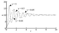
Fig. 4 Water level regulation using traditional adaptive law.

B. Switched Reset Adaptive Law

Assume we know $\| {\bar \theta - \theta^* } \| \le 0.1$.

Choosing ${V_1} = \frac{1}{2}{e^2}$ and $V = \frac{1}{2}{e^2} + \frac{1}{{2\gamma }}{\tilde \theta ^2}$, we have $c_1=c_2$ $=0.5, a=2, c_3=1$.

Since $\frac{1}{2}{e^2} \le \frac{1}{2}{e^2} + \frac{1}{{2\gamma }}{\tilde \theta ^2} \le \frac{1}{2}{e^2}(0) + \frac{1}{{2\gamma }}{\tilde \theta ^2}(0)$, noticing $e(0)=10$ and $\tilde \theta (0) \le 0.1$, we obtain $| e | \le \sqrt {100.01} $. Hence, $h={h_r}+e \le 10 + \sqrt {100.01} $. Consequently, we have $\Phi=\sqrt h\le4.5=M$.

Choose $l=2$, i.e., $c_4=0.5$, we have $\lambda=1$ and $B_{r}=\{ e|\left|e\right|\le0.9\}$. Choose $\bar \lambda =0.99$ and $\delta=0.01$. The condition of Theorem 3 is satisfied.

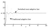
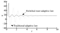
Using the same parameter as in the simulation of traditional adaptive law, we apply the adaptive law (34) in the simulation with $\gamma = 5$. The simulation result shown in Fig. 5 indicates that the switched reset adaptive law avoids large oscillations and improves the transient behavior. As is seen in Fig. 6, using the switched reset adaptive law, the oscillation magnitude of the control input also decreases obviously.

Fig. 5

	Download: JPG larger image
Fig. 5 Water level regulation using switched reset adaptive law.

Fig. 6

	Download: JPG larger image
Fig. 6 The control input using switched reset adaptive law.

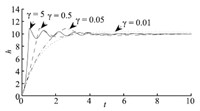
Fig. 7 shows the simulation result of switched reset adaptive control with $\gamma$ varying from 0.01 to 5. It appears that a larger $\gamma$ tends to result in a more rapid response. The resetting mechanism release us from the anxiety of large overshoot. When the adaptation is too slow, the chance of parameter over-adaptation is very small and the resetting mechanism may not be triggered, e.g., when $\gamma =0.01$ in this example. Even though, we cannot count on slow adaptation in avoiding large overshoots, because the control error also depends on the initial state of the system.

Fig. 7

	Download: JPG larger image
Fig. 7 Switched reset adaptive control using different $\gamma$.

${\bf Remark 15.}$ We have used the pre-estimate $\bar \theta =4.95$ as the initial estimate in the simulation, which is not demanded by the theorems. The results of this paper hold for any other selections of $\hat \theta(t_0)$.

A switched reset adaptive law has been proposed for a class of uncertain nonlinear systems. A known transient bound has been ensured outside a ball with asymptotical convergence reserved. Conditions for exponential decaying bound have been given with specified reaching time to a definite ball. Stability analysis has been provided using Lyapunov-like function. Simulation has been provided to demonstrate the effectiveness of the method.

The transient bound has been shown to exist outside a ball whose size is related to the accuracy of the pre-estimate. If we add an iterative parameter identification mechanism on line, the ball would vanish with the improving identification accuracy, which is our future study.