2. Beijing Institute of Electronic System Engineering, Beijing 100854, China;
3. School of Automation Science and Electrical Engineering, Beihang University, Beijing 100191, China
Airbreathing hypersonic vehicles (AHVs) have been studied broadly due to the prospects of high speed transportation and affordable space access for a long time. For the purpose of flight safety and high accuracy,control system design has become a core problem for AHV. However,the following characteristics of AHV make this problem full of challenges[1, 2, 3, 4, 5].
1) There are strong couplings between propulsive and aerodynamic forces,which are caused by the integrated configuration of the airframe and the scramjet engine.
2) The uncertainties of aerodynamic parameters[1] are derived from large-scale variations of altitude and velocity.
3) The immeasurable states exist in hypersonic condition.
In the past decades,amounts of work has been done for developing control system of hypersonic flight vehicle. Mainly,the control system design can be classified into two categories based on the linear and nonlinear models,respectively. For the controller design of the linearized dynamic models of hypersonic vehicles, several methods are adopted While considering the problems of different complexity,such as decentralized control[6], linear quadratic regulator (LQR) approach[7],gain scheduling method[8],etc. On the assumption that the fight dynamics at a certain point can be denoted by the linear combination of the model on adjacent design points,the linear parameter varying (LPV) model of hypersonic vehicle is proposed. Various methods are developed for LPV system of hypersonic vehicle[9, 10]. T-S fuzzy system based method is also adopted to synthesize controller for hypersonic vehicle based on linearized dynamical model[11]. Linearized dynamical model for hypersonic vehicle is obtained through Jacobian linearization under certain conditions,which brings loss of dynamic characteristic to some degree.
Actually,the hypersonic flight vehicle is a nonlinear system,and the controllers based on nonlinear model are more accurate than the linear. The nonlinear methods include feedback linearization[12, 13],sliding mode[14, 15],etc. Feedback linearization requires repetitive differentiations of system nonlinear terms,which is difficult to achieve in real world. Sliding mode method is easy to cause chattering of the input. At present,as a kind of convenient control design method for strict feedback nonlinear system,backstepping has received a lot of research attention for applications in hypersonic vehicle control area[16, 17].
However,the methods mentioned above require full information of the states,which limits their practical applications. In fact, the angle of attack (AOA) is difficult to be measured in hypersonic condition. Hypersonic aerodynamic heating decline the performance of the commonly used air-data sensors. Flush air-data sensor (FADS) is another instrument for AOA measurement,but when used in hypersonic condition,modeling of aerodynamic heating process is also a hard task,which is the fundamental problem of FADS[2].
Observer-based output feedback control is a feasible method for hypersonic vehicle[2, 13, 18] in the presence of immeasurable states. In [13],a sliding mode observer (SMO) is used to construct the immeasurable states. However,the observer is developed based on the exactly known parameters in the dynamic equations. When there exist parameters uncertainties,the equilibrium point of this observer is not the origin,which brings steady estimation errors. Besides,the controller is designed based on feedback linearization and sliding mode control. However, complex derivative signals of altitude and velocity are essential, but unavailable.
Reference [18] proposes a kind of robust output feedback scheme for linearized hypersonic vehicle model. The information used in the controller only includes velocity,altitude,pitch rate and normal acceleration,while the required state signals in the nominal controller are replaced by the signals from the full state observer.
Reference [2] proposes an output feedback controller combining backstepping and sliding mode observer. The stability of the closed-loop system and the convergence of the output tracking error are verified based on the small-gain theorem. However,parameter uncertainties are not considered,and the problem of "explosion of complexity" arising from the differentiation of the intermediate virtual control exists in [2]. Besides,the small-gain theorem holds only when tracking errors are out of certain range,so the stability proof is not complete.
A number of difficulties still exist in output feedback controller for hypersonic vehicle system.
1) The system cannot be exactly expressed in strict feedback form.
2) Forces and moment of hypersonic vehicle are the functions of AOA and its high order terms.
3) Altitude information cannot be used as unique information to estimate AOA because its precision is much lower than the measured values of pitch angle and pitch angle rate.
4) The aerodynamic coefficients are uncertain to some degree.
These four difficulties lead to the failure of commonly used high-gain observer or K-filter. Reference [19] solves a class of nonlinear systems output feedback tracking problem combining the modified high-gain observer and the adaptive backstepping controller,but the uncertainties are dominated by output-dependent functions,and the immeasurable states are constructed using the first state information which is also the output variable. The virtual control coefficients in [19] are ones,which is another advantage of output feedback controller design. Reference [20] proposes an output feedback control scheme for a class of stochastic nonlinear systems combining a kind of full-order observer and backstepping approach,in which the virtual control gains are also ones. Output feedback control for stabilization problem of nonlinear system is summarized in [21]. The control schemes above are not suitable for the hypersonic vehicle model.
In this paper,the objective is to construct a nonlinear output feedback tracking controller for hypersonic vehicle. The main contributions of this paper are summarized as follows.
1) The local characteristic of thrust and pitching moment with respect to AOA in the argument range is first validated. The advantage of this characteristic is discussed in Remark 1.
2) A reduced order observer is first proposed to estimate the value of immeasurable AOA based on the information of pitch angle and its rate.
3) The output feedback fuzzy dynamic surface technique[22] is first adopted for hypersonic vehicle control,which drives the trajectories of the velocity and altitude tracking errors into an arbitrarily small neighborhood of the origin. Fuzzy logic system method is used to compensate the effects of parameter uncertainties.
Besides these contributions,continuous hyperbolic tangent function is used in the virtual and actual control design to eliminate the effect of fuzzy estimation. Numerical simulations of various situations are presented. The maneuver is performed under several conditions to demonstrate that the control laws are valid for the entire flight envelope. It is shown that trajectory control is established for the closed-loop system even in the presence of uncertainties and immeasurable states in the vehicle model.
The reminder of this paper is organized as follows. The hypersonic vehicle longitudinal motion model is described in Section Ⅱ. In Section Ⅲ,the flight control system for hypersonic vehicles adopting the fuzzy reduced order observer and fuzzy dynamic surface technique is addressed. A comprehensive stability analysis is given for the closed-loop system. In Section IV,numerical simulations on the longitudinal hypersonic vehicle model are carried out to validate the proposed controller. Finally,brief concluding remarks end the paper in Section V.
Ⅱ. PLANT MODEL AND PROBLEM FORMULATIONThe hypersonic vehicle model considered in this study is the curve-fitted model (CFM) given by Fiorentini[16],where the complex forces and moment are approximated in curve-fitted form. The control inputs of this model are the elevator deflection angle and fuel-to-air ratio. The longitudinal dynamic equations are written as
| {˙h=Vsinγ,˙V=Tcosα−Dm−gsinγ,˙γ=L+TsinαmV−gVcosγ,˙α=−L+TsinαmV+Q+gVcosγ,˙θ=Q,˙Q=MIyy,¨ηi=−2ζiωi˙ηi−ω2iηi+Ni,i=1,2,3, | (1) |
| {T≈ˉqS[CT,Φ(α)Φ+CT(α)+CηTη],D=ˉqSCD(α,δe,η),L=ˉqSCL(α,δe,η),M=zTT+ˉqSˉcCM(α,δe,η), | (2) |
| {CT,Φ(α)=CΦα3Tα3+CΦα2Tα2+CΦαTα+CΦT+ΔCT,Φ,CT(α)=C3Tα3+C2Tα2+C1Tα+C0T+ΔCT,CL(α,δe)=CαLα+CδeLδe+C0L+CηLη+ΔCL,CD(α,δe)=Cα2Dα2+CαDα+Cδ2eDδ2e+CδeDδe+C0D+ CηDη+ΔCD,CM(α,δe)=Cα2Mα2+CαMα+CδeMδe+C0M+ CηMη+ΔCM,Cηj=[Cη1j 0 Cη2j 0 Cη3j 0], j=T,M,L,D,Nηi=[Nη1i 0 Nη2i 0 Nη3i 0],i=1,2,3. | (3) |
The rest of nomenclatures are revealed in Table Ⅰ. The admissible ranges of states and inputs are displayed in Table Ⅱ.
|
|
Table Ⅰ NOMENCLATURES OF HYPERSONIC VEHICLE |
|
|
Table Ⅱ ADMISSIBLE RANGES OF STATES,INPUTS,DYNAMIC PRESSURE,AND MACH NUMBER |
Remark 1. The CFM is derived from the true model (TM) in [3] by expressing T,L,D,M in the curve-fitted form. This manner is similar to the method of Parker[23]. The CFM can depict the TM with sufficient accuracy. All the dominant features including the coupling between thrust and aerodynamic forces,the effect of the thrust (engine) on the moment,the flexibility effect and the nonlinearity of force and moment are all retained in this model. Due to the lack of data for the TM,the CFM is taken as the simulation model to produce true states of AHV in this paper. The data of CFM can be found in [24].
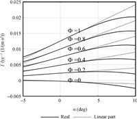
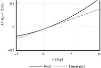
From equations (1)-(3),thrust T and moment M are expressed in nonlinear form. We calculate T for different Φ and α,and M for different α while the elevator angle is the trim value,and the relationships are depicted in Figs. 1 and 2.
|
Download:
|
| Fig. 1 T for different α and Φ | |
|
Download:
|
| Fig. 2 M for different α | |
It is obtained that T and M satisfy the locally Lipschitz condition with respect to AOA in the argument range according to Figs.\,1 and 2. Consequently,for the value of Φ and δe in the admissible range,T(α,Φ) and M(α,δe) satisfy the Lipschitz condition with some Lipschitz constants σT and σM as
| |T(α1,Φ)−T(α2,Φ)|≤σT|α1−α2|,|M(α1,δe)−M(α2,δe)|≤σM|α1−α2|,α1,α2∈Ωα, |
According to (1),the velocity is mainly controlled by the throttle setting Φ,while the change of the altitude is governed by the elevator deflection δe. Therefore,we separate the longitudinal dynamics into two subsystems,and design the velocity controller and altitude controller separately. The velocity is considered separately from the rest of dynamics,and the model is denoted as
| ˙V=fv+gvΦ, | (4) |
| x=[x1,x2,x3,x4]T=[h/hc,γ,θ,q]T. |
| ˙x1=g1(V)sinx2,˙x2=f2(x2,V)+g2(V)x3+w1(α,αref,δe,η),˙x3=g3x4,˙x4=f4(x2,x3,V)+g4(V)u+w2(α,αref,δe,,η), | (5-8) |
| g1(V)=V/hc, g2(V)=(CαLqS+kT1)/(mV),f2(x2,V)=f20(x2,V)−g2(V)×γ,f20(x1,V)=C0LqS/(mV)−g/V, g3=1,f4=[zT(kT2α+CcT)+ˉqSˉc(kMα+C0M)]/Iyy,g4=qSˉcCδeM/Iyy, u=δe,kT1=Cα3T(αref)3+Cα2T(αref)2+CαT(αref)+CcT,kT2=Cα3T(αref)2+Cα2Tαref+CαT,kM=Cα2Mαref+CαM. |
The goal of this study is to synthesize a controller using measurable state information realizing altitude and velocity tracking.
Remark 2. It can be concluded that w1 and w2 are mainly constituted by three parts,namely,the difference between αref and α,coefficient uncertainties and generalized elastic coordinates. From the locally Lipschitz characteristic of T and M,we can obtain that the first one can also be seen as coefficient uncertainty.
The following assumptions are made for developing the output feedback based control laws.
Assumption 1. The generalized elastic coordinate is mainly affected by AOA and is much less affected by δe.
Assumption 2. The reference signal hd(t) is a sufficiently smooth function of t,and hd(t),˙hd(t),¨hd(t) are bounded within a known compact set
| Ωhd={[hd,˙hd,¨hd]T:h2d+˙h2d+¨h2d≤h0}∈R3, |
Remark 3. Assumption 1 is made according to the scale of Nαi and Nδei; Nδei is much smaller than Nαi. Assumption 1 will be verified in the simulation.
Ⅲ. OUTPUT FEEDBACK DYNAMIC SURFACE CONTROLLERThe strategy chosen here is an output feedback controller based on dynamic surface control (DSC). First a fuzzy reduced order observer is designed for altitude loop to estimate AOA. Simultaneously,the estimated value of FPA is obtained based on the value of pitch angle and estimated value of AOA. Then,the dynamic surface control is applied using the estimated value of FPA,pitch angle,pitch angle as virtual control inputs,and the estimation error of FPA and uncertainties are considered as disturbances whose behavior must be dominated.
A. Fuzzy Logic Systems and Reduced Order Observer Design for Altitude LoopFirst we introduce the following useful lemma on fuzzy logic systems (FLSs).
Lemma 1[25] Let f(x) be a continuous function of vector x defined on a compact set U. Then for any constant ε>0,there exists the following FLSs:
| ˆf(x|ϑ)=ϑ∗Tφ(x), | (9) |
| supx∈U|ˆf(x|ϑ)−f(x)|≤ε, | (10) |
| ϑ∗=argminϑ∈Ω(supx∈U|ˆf(x|ϑ)−f(x)|). |
| φl(x)=n∏i=1μFli(xi)N∑l=1(∏ni=1μFli(xi)), |
| ˆwi(xb|ϑi)=ϑTiφi(xb). | (11) |
| ˆwi(x_b|ϑi)=ϑTiφi(x_b). | (12) |
| ϑ∗i=argminϑi∈Ωi(supxb∈Ubx_b∈U−b |ˆwi(xb|ϑ1)−wi(xb)|), | (13) |
| ε∗i=wi(xb)−ˆwi(x_b|ϑ∗i),εi=wi(xb)−ˆwi(x_b|ϑi). | (14-15) |
Assumption 3. With the boundedness of η,there exist known constants ε∗0i>0 and ε0i>0,such that |ε∗i|≤ε∗0i and |εi|≤ε0i (i=1,2).
A reduced order observer for AOA dynamics is formulated as
| {ˆα=ξ+Ly=ξ+l1θ+l2q,˙ξ=Mξ+Nδe+Ry+C=Mξ+Nδe+r1θ+r2q+C, | (16) |
| M=−ˉqSCαL+kT1mV−l2(zTkT2+ˉqSˉckM)Iyy,r1=l1=0,r2=(−ˉqSCαL+kT1mV−l2(zTkT2+ˉqSˉckM)Iyy)l2+1,N=−ˉqSCδeLmV−l2ˉqSˉcCδeMIyy,C=−ˉqSC0LmV+gV−l2(zTCcT+ˉqSˉcC0M)Iyy−ˆw1(x_b|ϑ1)−l2ˆw2(x_b|ϑ2). |
| ˙e=˙α−˙ˆα=−ˉqS(CαLα+C0L)+kT1αmV+q+gV−w1−[Mξ+Nδe+r1θ+r2q+C+l1q+l2Iyy(zT(kT2α+CcT)+ˉqSˉc(kMα+CδeMδe+C0M))+l2w2]=Me−ε1−ε2. | (17) |
The stability of the estimation error is given by the following proposition.
Proposition 1. By using the observer in (16),the estimation error boundedly converge to a small value,and it can be made small enough by |e(∞)|=(ε01+ε02)√1−(2M+1).
Proof. Consider the Lyapunov function candidate as
| Ve=12e2. | (18) |
| ˙Ve= e˙e=e(Me−ε1−ε2)≤Me2+(ε01+ε02)|e|≤(M+12)e2+(ε01+ε02)22≤(2M+1)Ve+(ε01+ε02)22. |
According to the differential inequality theory,there exists the following inequality by induction
| Ve(t)≤Ve(0)e(2M+1)t+∫t0e(2M+1)(t−τ)(ε01+ε02)22dτ, |
B. Controller Design for Altitude Loop In this section,an adaptive fuzzy controller and parameter adaptive laws are to be developed in the framework of the backstepping design and DSC technique so that all the signals in the closed-loop system are SUUB,and the tracking errors of altitude are as small as desired.
Step 1. Define the dynamic surface error (tracking error) as z1:=x1−hd,whose time derivative while considering (5) is
| ˙z1=g1(V)ˉx2−˙hd. | (19) |
Although the precision of altitude signal is not high enough to estimate AOA,it can be taken into altitude tracking error calculation. The nominal command of virtual control variable ˉx2 is designed as
| ˉxref02=1g1(V)(−k1z1+˙hd). | (20) |
| ˙ˉxref2=−T2(ˉxref2−ˉxref02),ˉxref2(0)=ˉxref02(0), | (21) |
Step 2. Define the dynamic surface equation in Eq. as z2:=sinˆx2−ˉxref2,whose dynamics can be calculated by (6),i.e.,
| ˙z2=cos(ˆx2)[f2(x2,V)+g2(V)x3+w1(xb)+˙e]−˙xref2, | (22) |
| g2(V)xref03=1cos(ˆx2)[−k2z2−g1z1−(ε∗01+ε01+ε02)tanh(z2ε2)+˙ˉxref2]−f20(x2,V)+g2(V)׈γ−ˆw1(x_b|ϑ1). | (23) |
| ˙xref3=−T3(xref3−xref03),xref3(0)=xref03(0), | (24) |
Step 3. Define dynamic surface as z3:=x3−xref3,its dynamics can be calculated from (6),i.e.,
| ˙z3=x4−˙xref3, |
| xref04=−k3z3+˙xref3−z2cos(ˆx2)g2(V). | (25) |
| ˙xref4=−T4(xref4−xref04),xref4(0)=xref04(0). | (26) |
| ˙z4=f4(x2,x3,V)+g4(V)u+w2(xb)−˙xref4. | (27) |
| g4(V)u=−k4z4−f4(ˆx2,x3,V)+˙xref4−z3−ˆw2(x_b|ϑ2)− ε∗02tanh(z4ε4). | (28) |
| ˙zV=ˆfv+ˆgvΦ+dv−˙Vd, | (29) |
| {E11=Z11−V,˙Z11=Z12+ˆfv−β11E11+ˆgvΦ,˙Z12=−β12fal(E11,λv,εv), | (30) |
| fal(E11,λv,εv)={|E11|λvsgn(E11),|E11|>εv,E11ε1−λvv,others. | (31) |
| Φ=ˆg−1v(V)(−kvzV−ˆfv−Z12+˙Vd). | (32) |
D. Stability and Performance Analysis In this section,we will prove that by using the proposed output feedback dynamic surface control scheme,the semiglobal stability of the closed-loop system can be guaranteed. Furthermore,the tracking performance can be achieved through tuning control coefficients under an initialization error constraint condition.
Define the error between the nominal and actual values of virtual control variable as
| δ2=xref2−xref02,δ3=xref3−xref03,δ4=xref4−xref04. |
| ˙z1=g1(V)x2−˙hd=g1(V)(e+z2+δ2+xref02)−˙hd=−k1z1+g1(V)(e+z2+δ2),˙z2=−k2z2+cos(ˆx2)g2(V)(z3+δ3+e)+cos(ˆx2)×[w1(xb)−ˆw1(x_b|ϑ1)]+cos(ˆx2)˙e−g1z1−(ε∗01+ε01+ε02)tanh(z2ε2),˙z3=−k3z3+z4+δ4−z2g2(V),˙z4=−k4z4+(zTkT2+ˉqSˉckM)eIyy+w2(xb)−ˆw2(x_b|ϑ2)−z3−ε∗02tanh(z4ε4). | (33-36) |
| δi˙δi=δiTi(xref0i−xrefi)−δi˙xref0i≤−Tiδ2i+|δi|ψi(z1,z2,z3,z4,δ1,δ2,δ3,hd,˙hd,¨hd), | (37) |
By defining ˜ϑ1=ϑ1−ϑ1∗,˜ϑ2=ϑ2−ϑ2∗,then the FLS estimation error can be denoted as
| wi(xb)−ˆwi(x_b|ϑi)=[wi(xb)−ˆwi(x_b|ϑ∗i)]+[ˆwi(x_b|ϑ∗i)−ˆwi(x_b|ϑi)]=ε∗i−ϑTiφi(x_b). | (38) |
The following lemma will be used in stability analysis.
Lemma 2[28] For any constant ε>0,χ∈R,the following inequality holds:
| 0≤|χ|−χtanh(χε)≤kpε, |
We conclude the stability of the closed-loop altitude subsystem in the following theorem.
Theorem 1. Given motion equations (6)~(8) for the altitude loop of hypersonic flight vehicle,the proposed dynamic surface controller (28),together with the FLSs estimator (16),there exist proper positive numbers ki,Tj (i=1,2,3,4,j=2,3,4) and a negative number M,such that all signals of the closed-loop altitude system are uniformly bounded, and the altitude tracking error z1 converges to a residual set that can be made arbitrarily small by properly choosing some design parameters.
Proof. Define the Lyapunov function candidate as
| Val=124∑i=1z2i+124∑j=2δ2j+122∑k=1Γ−1ϑk˜ϑTk˜ϑk+12e2. | (39) |
| ˙Val=z1[−k1z1+g1(V)(e+z2+δ2)]+z2[−k2z2+cos(ˆx2)g2(V)(z3+δ3+e)+cos(ˆx2)×[w1(xb)−ˆw1(x_b|ϑ1)]−g1z1+cos(ˆx2)˙e−(ε∗01+ε01+ε02)×tanh(z2ε2)]+z3[−k3z3+z4+δ4−z2cos(ˆx2)g2(V)]+z4[−k4z4+(zTkT2+ˉqSˉckM)eIyy+w2(xb)−ˆw2(x_b|ϑ2)−z3−ε∗02tanh(z4ε4)]+4∑j=2δj˙δj+2∑k=1Γ−1ϑk˜ϑTk˙˜ϑk+e˙e. |
By simplifying the equation,the derivative of Lyapunov function is transformed into
| ˙Val=z1[−k1z1+g1(V)(e+δ2)]+z2[−k2z2+cos(ˆx2)g2(V)(z3+δ3+e)+cos(ˆx2)×[w1(xb)−ˆw1(x_b|ϑ1)]+cos(ˆx2)˙e−(ε∗01+ε01+ε02)×tanh(z2ε2)]+z3[−k3z3+δ4]+z4[−k4z4+(zTkT2+ˉqSˉckM)eIyy+w2(xb)−ˆw2(x_b|ϑ2)−ε∗02tanh(z4ε4)]+4∑j=2δj˙δj+2∑k=1Γ−1ϑk˜ϑTk˙˜ϑk+e˙e=−k1z21+g1(V)z1(e+δ2)−k2z22+g2(V)cos(ˆx2)z2×(δ3+e)+z2cos(ˆx2)(ε∗1−˜ϑT1φ1(x_b))+z2cos(ˆx2)×(Me−ε1−ε2)−(ε∗01+ε01+ε02)z2tanh(z2ε2)−k3z23+z3δ4−k4z24+ˉkMez4+z4(ε∗2−˜ϑT2φ2(x_b))−ε∗02z4tanh(z4ε4)+4∑j=2δj˙δj+2∑k=1Γ−1ϑk˜ϑTk˙˜ϑk+e˙e, |
| {g1(V)z1e≤12(g21(V)e2+z21),g1(V)z1δ2≤12(z21+g21(V)δ22),g2(V)cos(ˆx2)z2δ3≤12(z22+g22(V)δ23),g2(V)cos(ˆx2)z2e≤12(e2+g22(V)z22),z2cos(ˆx2)Me≤12(M2z22+e2),z3δ4≤12(z23+δ24),ˉkMez4≤12(ˉk2Mz24+e2). | (41) |
| ˙Val⩽−k1z21+12(g21(V)e2+z21)+12(z21+g21(V)δ22)k2z22+12(z22+g22(V)δ23)+12(e2+g22(V)z22)+z2ε∗1+z2˜ϑT1φ1(x_b)+12z2˜ϑT1φ1(xb)2(M2z22+e2)+|z2(ε01+ε02)|− |
| (ε∗01+ε01 + ε02)z2tanh(z2ε2)−k3z23+12(z23+δ24)−k4z24+12(ˉk2Mz24+e2)+z4ε∗2−ε∗02z4tanh(z4ε4)+z4ϑT2φ2(x_b)+4∑j=2δj˙δj+2∑k=1Γ−1ϑk˜ϑTk.˜ϑk+e˙e⩽ |
| −(k1−1)z21+12g21(V)e2+12g21(V)δ22−(k2−12−12g22(V))z22+12g22(V)δ23+12e2+|z2(ε∗01+ε01+ε02)|−(ε∗01+ε01 + ε02)z2tanh(z2ε2)+z2˜ϑT1φ1(x_b)−Γ−1ϑ1˜ϑT1.ϑ1+12(M2z22+e2)− |
| (k3−12)z23+12δ24−k4z24+12(ˉk2Mz24+e2)+|z4ε∗02|−ε∗02z4tanh(z4ε4)+z4ϑT2φ2(x_b)−Γ−1ϑ2ϑT2.ϑ2+4∑j=2(−Tiδ2i+|δi|ψi)+e(Me−ε1−ε2). | (42) |
| ˙ϑ1=Γϑ1(−z2φ1(xb)+β1ϑ1), | (43) |
| ˙ϑ2=Γϑ2(−z4φ2(xb)+β2ϑ2). | (44) |
| −β1ϑT1ϑ1≤−β1‖ϑ1‖22+β1‖ϑ∗1‖22, | (45) |
| −β2ϑT2ϑ2≤−β2‖ϑ2‖22+β2‖ϑ∗2‖22. | (46) |
| ˙Val≤−(k1−1)z21−(k2−12−12g22(V)−12M2)z22−(k3−12)z23−(k4−12ˉk2M)z24−(T3−12g22(V))δ23+(M+12g21(V)+32+ε01+ε022ς2e)e2+4∑j=2|δi|ψi−(T2−12g21(V))δ22−(T4−12)δ24−β1‖ϑ1‖22−β2‖ϑ2‖22+2kpς+ς2e2+β2‖ϑ∗2‖22+β1‖ϑ∗1‖22. | (47) |
Define the following sets:
| A:={(hd,˙hd,¨hd):h2d+˙h2d+¨h2d≤h0}, |
| B:={(z1,z2,z3,z4,δ2,δ3,δ4):z21+z22+z23+z24+δ22+δ23+δ24≤p}, |
| |δj|ψj≤|δj|Mψj≤(δ2jM2ψj2ςM+ςM2),j=2,3,4, | (48) |
| ˙Val≤−(k1−1)z21−(k2−12−12g22(V)−12M2)z22−(k3−12)z23−(k4−12ˉk2M)z24−(T3−12g22(V)−M2ψ32ςM)δ23+(M+12g21(V)+32+ε01+ε022ς2e)e2−(T2−12g21(V)−M2ψ22ςM)δ22−(T4−12−M2ψ42ςM)δ24−β1‖ϑ1‖22−β2‖ϑ2‖22+3ςM2+2kpς+ς2e2+β2‖ϑ∗2‖22+β1‖ϑ∗1‖22. | (49) |
| {k1>1,k2>12+12g22(V)+12M2,k3>12, k4>12ˉk2M, T2>12g21(V)+M2ψ22ςM,T3>12g22(V)+M2ψ32ςM, T4>12+M2ψ42ςM,M<−12g21(V)−32−ε01+ε022ς2e. | (50) |
| ˙Val≤−2α0Val+ε0, | (51) |
| α0=min{(k1−1),(k2−12−12g22(V)−12M2),(k3−12),(k4−ˉk2M2),(T4−12−M2ψ42ςM),β1Γϑ1,(T3−12g22(V)−M2ψ32ςM),(T2−12g21(V)−M2ψ22ςM),−(M+g21(V)2+32+ε01+ε022ς2e),β2Γϑ2},ε0=3ςM2+2kpς+ς2e2+β1‖ϑ∗1‖22+β2‖ϑ∗2‖22. |
| Val(t)≤Val(0)e−2α0t+∫t0e−2α0(t−τ)ε0dτ. | (52) |
The extended state observer can estimate the disturbance dv in finite time,and the estimation error ˜dv=dv−Z12 can be extremely small[26, 27],so the tracking error dynamics can be approximated by ˙zV=−kvzV,which guarantees the stability of velocity loop and convergence of velocity tracking error.
The generalized elastic coordinate system can be treated as a disturbance to the rigid-body system[29]. Theorem 1 shows that the closed-loop altitude system has strong disturbance attenuation ability. Velocity loop also possesses high disturbance attenuation ability with the help of extended state observer. Thus,the boundedness of generalized elastic coordinate can guarantee the stability of rigid system. With Assumption 1,the dynamics of generalized elastic coordinate is mainly affected by AOA,so the boundedness of AOA can guarantee the stability of the structure elastic system from the system dynamics in (1). Thus,the stability of the whole system can be guaranteed by the small-gain theorem[30].
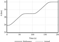
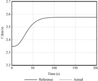
Ⅳ. SIMULATIONSTo show the performance of the controllers proposed in previous sections,simulations have been performed on the fully nonlinear vehicle model described by (1). The vehicle is desired to track the velocity and altitude references initialized at V0 = 2 347.6 m ⋅s−1,h0 = 25 908 m, γ0 = 0 deg. The reference commands of velocity and altitude are generated by filtering step reference commands using two second-order pre-filters with natural frequency ωf=0.03 rad/s and damping factor ξf=0.95. Reference hd(t) is generated to let the vehicle climb 6.1 km in about 180 s in two steps,whereas the velocity reference is one step signal with the increase of 228.6 m/s.
The simulations are accomplished in three steps,corresponding to the nominal model,uncertain model with compensation,and the comparisons with other schemes. The compensation-control involves fuzzy logic compensation and uncertainty estimation error compensation.
The parameters used in the controllers of all simulations are shown in Table Ⅲ. The first simulation is only for the nominal model, indicating the uncertainties are ignored,that is to say,w1=w2=0. The reference signals of virtual control variables are chosen according to equations (20),(23) and (25),and the control input is computed from (28). In this study,the constraints on states and inputs are dealt with indirectly by tuning the controller gains,including the parameters of the pre-filter and dynamic surface gain ki (i=1,⋯,4). The selection of gain ki should make the inner loop respond quicker than the outer loop. The controller gains used in all simulations are shown in Table Ⅲ.
|
|
Table Ⅲ CONTROLLER PARAMETERS |
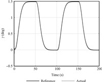
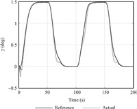
Figs. 3 and 4 confirm that the controllers provide stable tracking of the reference trajectories of altitude and velocity and exact convergence to the reference command. The flight-path angle reference command,as depicted in Fig. 5 is well tracked. The flight-path angle is smaller than 1.5 deg during the whole process, which validates the small angle assumption used in Section II.
|
Download:
|
| Fig. 3 The tracking curve of altitude command. | |
|
Download:
|
| Fig. 4 The tracking curve of velocity command. | |
|
Download:
|
| Fig. 5 The tracking curve of FPA. | |
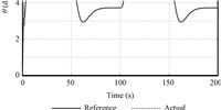
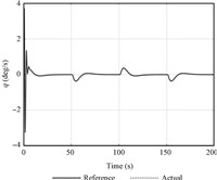
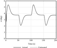
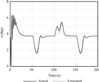
Figs. 6 and 7 show the tracking performance of the virtual control variables of pitch angle and its rate. The virtual control commands are smooth within their bounds,and are nicely tracked. The estimation curve of AOA is given in Fig. 9,which shows the good performance of the proposed estimator.
|
Download:
|
| Fig. 6 The tracking curve of pitch angle. | |
|
Download:
|
| Fig. 7 The tracking curve of pitch angle rate. | |
|
Download:
|
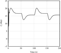
| Fig. 8 The curve of elevator deflection. | |
|
Download:
|
| Fig. 9 The estimate in curve of AOA. | |
According to the simulation results in nominal condition,it is clear that even though the exact information on AOA is immeasurable,the proposed adaptive fuzzy output feedback controller guarantees both the stability and good tracking performance of the closed-loop system.
The second simulation is performed for the system with uncertainties. The references of velocity,altitude,and flight-path angle are the same as those in the first simulation. It is assumed that the true value of some aerodynamic parameters including CαL,Cα2D,CαM are unknown and different from the nominal value within the tolerance of 5%. Additionally,the mass and moment of inertia vary by 10% of their nominal values. The simulation is conducted considering the effects of the generalized elastic coordinates.
The fuzzy weighting values are computed with update laws (39) and (40). The gains of the update laws are selected as Tϑ1=80,β1=0.05,Tϑ2=140,β2=0.05. Gaussian membership function is used,and the variances should be in the suitable range,corresponding to the partitioning points selected. From Remark 1,the uncertainty from the difference between αref and α can also be seen as coefficient uncertainty,so w1 and w2 can be predigested as the functions of α,δe and η. In the FLSs,we use ˆα,δe and η∗ as inputs. The partitioning points are chosen as -4,-1,2, 5,8 deg,and -20,-15,-10,-5,0,5,10,15,20 deg for ˆα and δe,respectively. The partitioning points for η are selected according to the scale of each generalized elastic coordinate which can be estimated by the trim value. In this simulation,we select −1.5 to 1.5 with the interval of 0.3 for η1,−0.6 to 0.6 with the interval of 0.06 for η2 and −0.12 to 0.12 with the interval of 0.03 for η3. The fuzzy membership functions for ˆα are given as follows,and the fuzzy membership functions for δe and η are similar to ˆα:
| μF11(ˆα)=11+e80/(ˆα+4/57.3),μF21(ˆα)=e−(ˆα+157.30.04)2,μF31(ˆα)=e−(ˆα−257.30.04)2,μF41(ˆα)=e−(ˆα−557.30.04)2,μF51(ˆα)=11+e−80/(ˆα−857.3). |
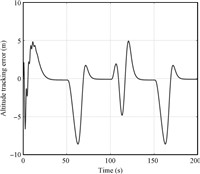
It can be seen that the tracking error of altitude remains very well behaved in the presence of model uncertainties. The tracking errors remain remarkably small during the entire maneuver,and vanish asymptotically. The good performance of the fuzzy compensators are demonstrated. In fact,extensive studies are performed on changing the fuzzy membership functions and weighing update gains for exact estimation of model uncertainties.
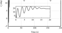
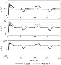
The effect of δe on the generalized elastic coordinate is also analyzed in this simulation. It can be seen from Fig. 15 that the effect of δe is much smaller than that of other parts,mainly the angle of attack.

|
Download:
|
| Fig. 10 The tracking curve of altitude command with uncertainty | |
|
Download:
|
| Fig. 11 The tracking error of altitude | |
|
Download:
|
| Fig. 12 The tracking curve of altitude command with uncertainty. | |
|
Download:
|
| Fig. 13 The tracking error of altitude. | |
|
Download:
|
| Fig. 14 The estimation curve of AOA. | |
|
Download:
|
| Fig. 15 The curve of elevator deflection | |
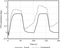
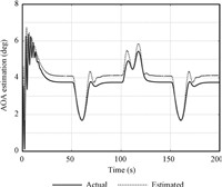
Reference [13] proposes a kind of sliding mode observer to estimate FPA and AOA. The observer and controller are designed separately. In this paper,we will give the off-line estimation results of SMO,and make a comparison with our proposed observer. The design parameters of SMO are selected according to the principle given in [13]. The simulation is conducted in the same uncertainty condition as in the second simulation.
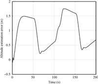
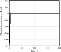
The simulation results are given in Figs. 16~19. From Fig. 17,it can be seen that the estimation error of pitch rate converges to zero quickly,but this do not ensure the convergence of AOA estimation error,which can be seen from Fig. 19. The existence of uncertainty changes the origin of the observer,which make estimation value of AOA cannot converge to its true value. The estimation error of AOA affects the convergence of altitude and FPA,which can be seen from Figs. 16 and 18. In the proposed method of this paper,the observer and controller are designed in associated manner. The uncertainty is estimated by FLSs whose parameters are adaptively tuned in the controller. Thus,the uncertainty is well compensated in the estimator. Besides,the stability analysis of observer can be proved in theory.
|
Download:
|
| Fig. 16 Altitude estimation error with SMO. | |
|
Download:
|
| Fig. 17 Pitch estimation error with SMO. | |
|
Download:
|
| Fig. 18 FPA estimation curve with SMO. | |
|
Download:
|
| Fig. 19 AOA estimation curve with SMO. | |
Remark 4. Comparing to state feedback based back-stepping control scheme[16, 17] for the hypersonic vehicle,the proposed scheme in this paper is constructed using limited state information, but achieves relatively good tracking performance of velocity and altitude. Additionally,dynamic surface technique used in this paper avoids the “complexity explosion” of backstepping control.
Ⅴ. CONCLUSIONThe usual air-data measurement system cannot work well due to hypersonic aerodynamic heating. Thus,output feedback controller is an essential issue for generic airbreathing hypersonic flight vehicle. A novel output feedback control scheme is developed in this paper. Estimated AOA value is acquired through a reduced order observer only using pitch angle and its rate information. The control system is constructed based on the AOA signal from observer. Dynamic surface technique is used in controller design for avoiding “complexity explosion” of traditional backstepping control. Fuzzy logic based compensator is used in the controller to dispose the inaccuracy and uncertainty of the model. Different from the existing output feedback controller in the literature, this scheme not only uses limited information,but also takes model uncertainty into consideration,which greatly strengthen the robustness of control system. At last,simulation results demonstrate the good performance of the proposed method.
| [1] | Chavez F R, Schmidt D K. Uncertainty modeling for multivariablecontrol robustness analysis of elastic high-speed vehicles. Journal of Guidance, Control, and Dynamics, 1999, 22(1):87-95 |
| [2] | Zong Q, Ji Y H, Zeng F L, Liu H L. Output feedback backstepping control for a generic hypersonic vehicle via small gain theorem. Aerospace Science and Technology, 2012, 23(1):409-417 |
| [3] | Bolender M A, Doman D B. Nonlinear longitudinal dynamical model of an air-breathing hypersonic vehicle. Journal of Spacecraft and Rockets, 2007, 44(2):374-387 |
| [4] | Sun Chang-Yin, Mu Chao-Xu, Yu Yao. Some control problems for near space hypersonic vehicles. Acta Automatica Sinica, 2013, 39(11):1901-1913(in Chinese) |
| [5] | Bao Wei-Min. Present situation and development tendency of aerospace control techniques. Acta Automatica Sinica, 2013, 39(6):609-702(in Chinese) |
| [6] | Dickeson J J, Rodriguez A A, Sridharam S, Benavides J, Soloway D. Decentralized control of an air-breathing scramjet-powered hypersonic vehicle. In:Proceedings of the 2009 AIAA Guidance, Navigation and Control Conference. Chicago, IL:AIAA, 2009. AIAA-2009-6281 |
| [7] | Groves K P, Sigthorsson D O, Serrani A, Yurkovich S, Bolender M A, Doman D B. Reference command tracking for a linearized model of an air-breathing hypersonic vehicle. In:Proceedings of the 2005 AIAA Guidance, Navigation, and Control Conference. San Francisco, CA:AIAA, 2005. AIAA-2005-6144 |
| [8] | Lind R, Buffington J, Sparks A. Multi-loop aeroservoelastic control of a hypersonic vehicle. In:Proceedings of the 1999 AIAA Guidance, Navigation, and Control Conference. Portland, OR:AIAA, 1999. AIAA-99-4123 |
| [9] | Rick L. Linear parameter-varying modeling and control of structural dynamics with aerothermoelastic effects. Journal of Guidance, Control, and Dynamics, 2002, 25(4):733-739 |
| [10] | Wilcox Z D, Mackunis W, Bhat S, Lind R, Dixon W E. Lyapunov-based exponential tracking control of a hypersonic aircraft with aerothermoelastic effects. Journal of Guidance, Control, and Dynamics, 2010, 33(4):1213-1224 |
| [11] | Hu X, Wu L, Hu C, Gao H. Fuzzy guaranteed cost tracking control for a flexible air-breathing hypersonic vehicle. IET Control Theory and Applications, 2012, 69(4):1238-1249 |
| [12] | Wang Q, Stengel R F. Robust nonlinear control of a hypersonic aircraft. Journal of Guidance, Control, and Dynamics, 2000, 23(4):577-585 |
| [13] | Xu H J, Mirmirani M D, Ioannou P A. Adaptive sliding mode control design for a hypersonic. Journal of Guidance, Control, and Dynamics, 2004, 27(5):829-838 |
| [14] | Hu X X, Wu L G, Hu C H, Gao H J. Adaptive sliding mode tracking control for a flexible air-breathing hypersonic vehicle. Journal of the Franklin Institute, 2012, 349(2):559-577 |
| [15] | Gao G, Wang J Z. Reference command tracking control for an airbreathing hypersonic vehicle with parametric uncertainties. Journal of The Franklin Institute, 2013, 350(5):1155-1188 |
| [16] | Fiorentini L, Serrani A, Bolender M, Doman D B. Nonlinear robust adaptive control of flexible air-breathing hypersonic vehicles. Journal of Guidance, Control, and Dynamics, 2009, 32(2):401-416 |
| [17] | Bialy B J, Klotz J, Curtis J W, Dixon W E. An adaptive backstepping controller for a hypersonic air-breathing missile. In:Proceedings of the 2012 AIAA Guidance, Navigation and Control Conference. Minneapolis, MN:AIAA, 2012. AIAA-2012-4468 |
| [18] | David O S, Pete J, Andrea S. Robust linear output feedback control of an airbreathing hypersonic vehicle. Journal of Guidance, Control, and Dynamics, 2008, 31(4):1052-1066 |
| [19] | Zhang X, Lin Y. Adaptive output feedback tracking for a class of nonlinear systems. Automatica, 2012, 48(9):2372-2376 |
| [20] | Fan H J, Han L X., Wen C Y, Xu L. Decentralized adaptive outputfeedback controller design for stochastic nonlinear interconnected systems. Automatica, 2012, 48(11):2866-2873 |
| [21] | Jiang Zhong-Ping, Huang Jie. Stabilization and output regulation by nonlinear feedback:a brief overview. Acta Automatica Sinica, 2013, 39(9):1389-1401(in Chinese) |
| [22] | Tong S C, Li Y M, Feng G, Li T S. Observer-based adaptive fuzzy backstepping dynamic surface control for a class of MIMO nonlinear systems. IEEE Transactions on Systems, Man, and Cybernetics-Part B:Cybernetics, 2011, 41(12):1124-1135 |
| [23] | Parker J T, Serrani A, Yurkovich S, Bolender M A, Doman D B. Controloriented modeling of an air-breathing hypersonic vehicle. Journal of Guidance, Control, and Dynamics, 2007, 30(3):856-869 |
| [24] | Fiorentini L. Nonlinear Adaptive Controller Design for Air-Breathing Hypersonic Vehicles[Ph. D. dissertation], The Ohio State University, USA, 2010. |
| [25] | Tong S C, Li Y M, Feng G, Li T S. Observer-based adaptive fuzzy backstepping dynamic surface control for a class of non-linear systems with unknown time delays. IET Control Theory and Applications, 2011, 12(5):1426-1438 |
| [26] | Han J Q. From PID to active disturbance rejection control. IEEE Transactions on Industrial Electronics, 2009, 56(3):900-906 |
| [27] | Xia Y Q, Zhu Z, Fu M Y, Wang S. Attitude tracking of rigid spacecraft with bounded disturbances. IEEE Transactions on Industrial Electronics, 2011, 58(2):647-659 |
| [28] | Chen M, Ge S S, Ren B B. Adaptive tracking control of uncertain MIMO nonlinear systems with input constraints. Automatica, 2011, 47(3):452-465 |
| [29] | Sun H F, Yang Z L, Zeng J P. New tracking-control strategy for airbreathing hypersonic vehicles. Journal of Guidance, Control, and Dynamics, 2013, 36(3):846-859 |
| [30] | Jiang Z P, Teel A R, Praly L. Small-gain theorem for ISS systems and application. Mathematics of Control, Signals, and Systems, 1994, 7(2):95-120 |
 2015, Vol.2
  Fig. 1


