Ⅰ. INTRODUCTION

ADAPTIVE control has been used with success in a number of flight control applications. In certain situations,fast adaptation is needed in order to improve tracking performance rapidly when a system is subject to large uncertainty such as structural damage to an aircraft that could cause rapid changes in system dynamics. In these situations,adaptive control needs to be able to adapt quickly by the use of large adaptive gain in order to reduce the tracking error as fast as possible. However,fast adaptation in adaptive control can result in high frequency oscillations which can excite unmodeled dynamics that could adversely affect stability of an adaptive law^[1]. Poor robustness to unmodeled dynamics,time delay,and exogenous disturbances due to high gain adaptive control is well-known. Thus,in general there exists a delicate balance between performance and robustness. A large adaptive gain can generally improve tracking performance but usually at the expense of robustness.

To address the lack of robustness of the standard model-reference adaptive control,the two well-known robust modification methods in adaptive control,namely; the $\sigma$ modification^[2] and $e$ modification^[3],have been used extensively in adaptive control. Recent years have seen a surge in many new adaptive control methods such as the $\mathcal{L}_{1}$ adaptive control^{[4, 5]},adaptive loop recovery^[6],Kalman filter adaptive control^[7],derivative-free adaptive control^[8],command governor-based adaptive control^[9], concurrent learning adaptive control^[10],least-squares model-reference adaptive control^[11],composite model-reference adaptive control^[12],and optimal control modification^{[13, 14]}; just to name a few. In terms of addressing fast adaptation,the $\mathcal{L}_{1}$ adaptive control has gained a considerable attention due to its ability to achieve robustness with fast adaptation for a given a priori bound on the uncertainty. The existence of theoretical bounds on the transient performance and time delay margin of the $\mathcal{L}_{1}$ adaptive control enables it to address one of the current challenges in verification and validation: the lack of theoretically justifiable metrics^[15]. One of the key features of the $\mathcal{L}_{1}$ adaptive control is the existence of a linear input-output mapping with fast adaptation which helps to address the problem with predictability of nonlinear control^{[4, 5]}.

The optimal control modification has been developed using an optimal control framework to minimize the $\mathcal{L}_{2}$ norm of the tracking error bounded away from the origin by some lower bound^[13]. By increasing the lower bound,robustness can be improved by trading off with tracking performance. A number of extensions have been developed for the optimal control modification method. In the presence of actuator rate limiting,a time-scale separation principle is applied to the method to decouple the slow-fast system via the singular perturbation^[16]. This approach improves tracking performance in the presence of slow actuator dynamics. The optimal control modification method has also been used in conjunction with the newly developed derivative-free adaptive control^[17].

In terms of applications and validation,the optimal control modification method has been demonstrated in many flight environments ranging from low-fidelity desktop simulations to high-fidelity piloted motion-based flight simulations and flight testing on a piloted aircraft. For desktop simulations,the optimal control modification method has been applied to various aircraft models including NASA generic transport model (GTM) with damaged flight dynamics^[13] and aeroelastic longitudinal dynamics^[18],a general aviation aircraft^[19],and a NASA F/A-18A aircraft model^[20]. In 2009,a piloted flight simulation study has been conducted in a motion-based flight simulator at NASA Ames Research Center participated by eight NASA test pilots. Favorable Cooper-Harper ratings by the NASA test pilots have been noted with the optimal control modification adaptive law^{[21, 22]}. Subsequently,a series of flight experiments were conducted in late 2010 and early 2011 onboard a NASA F/A-18A test aircraft at NASA Dryden Flight Research Center to evaluate the effectiveness of the optimal control modification method with normalization^[23]. The flight test results show that the optimal control modification method offers the potential for flight control performance improvements under certain degraded flight control characteristics^{[24, 25]}.

In certain situations,the control effectiveness of a control system may be impaired due to failures. When an uncertainty exists in the control input,the system can undergo significant changes in its closed-loop characteristics that can compromise stability and performance of the control system. The control signal must be modified accordingly to produce achievable dynamics in the presence of the reduced control effectiveness. A new approach based on the optimal control modification adaptive law has been developed to address this issue. A parallel predictor model is constructed to relate the predictor error to the estimation error of the control effectiveness matrix. In this work,we will develop an optimal control modification adaptive control approach that seeks to minimize a bi-objective linear quadratic cost function of both the tracking error norm and the predictor error norm simultaneously. The resulting adaptive laws for the parametric uncertainty and control effectiveness uncertainty are dependent on both the tracking error and the predictor error,while the adaptive laws for the feedback gain and command feedforward gain are only dependent on the tracking error. In this context,the new adaptive law may be somewhat similar to the composite model-reference adaptive control^[12],but there also exists a significant difference in that the optimal control modification term that provides robustness to adaptive control does not exist in composite model-reference adaptive control and is derived from the optimal control formulation.

Ⅱ. BI-OBJECTIVE OPTIMAL CONTROL MODIFICATION ADAPTIVE LAWS

Consider the following nonlinear plant with control input uncertainty,matched uncertainty,and unmatched disturbance

\begin{align} \dot{x}=Ax+B\Lambda\left[u+\Theta^{*{\rm T}}\Phi\left(x\right)\right]+w,\label{1} \end{align}

(1)

where $x\left(t\right)\in{\bf R}^{n}$ is a state vector, $u\left(t\right)\in{\bf R}^{m}$ is a control vector,$A\in{\bf R}^{n\times n}$ is known,$B\in{\bf R}^{n\times m}$ is also known such that $\left(A,B\right)$ is controllable, $\Lambda=\Lambda^{\rm T}>0\in{\bf R}^{m\times m}$ is a constant unknown diagonal matrix with diagonal elements that represents a control input uncertainty,$\Theta^{*}\in{\bf R}^{p\times m}$ is a constant and unknown matrix that represents a matched parametric uncertainty,$\Phi\left(x\right)\in{\bf R}^{p}$ is a vector of known bounded regressors,and $w\left(t\right)\in{\bf R}^{n}$ is an unmatched bounded disturbance with bounded time derivative, i.e.,$\sup_{\forall t}\left\Vert w\right\Vert \le w_{0}$ and $\sup_{\forall t}\left \Vert \dot{w}\right\Vert \le\delta_{0}$.

A nominal fixed-gain controller is designed to stabilize the nominal plant which does not have uncertainty,i.e.,$\Lambda=I$ and $\Theta^{*}=0$,and to enable it to track a reference command signal $r\left(t\right)$ as follows:

\begin{align} \bar{u}=\bar{K}_{x}x+\bar{K}_{r}r, \end{align}

(2)

where $r\left(t\right)\in{\bf R}^{r}$ is a bounded reference command signal,such that $A+B\bar{K}_{x}\in{\bf R}^{n\times n}$ is Hurwitz,and $B\bar{K}_{r}\in{\bf R}^{n\times r}$.

The closed-loop nominal plant without uncertainty is then used to specify a reference model

\begin{align} \dot{x}_{m}=A_{m}x_{m}+B_{m}r, \end{align}

(3)

where $x_{m}\left(t\right)\in{\bf R}^{n}$ is a reference state vector,$A_{m}=A+B\bar{K}_{x}$,and $B_{m}=B\bar{K}_{r}$.

In the presence of both the control input uncertainty and matched uncertainty due to $\Lambda$ and $\Theta^{*}$,an adaptive controller is designed as

\begin{align} u=K_{x}\left(t\right)x+K_{r}\left(t\right)r-\Theta^{\rm T}\left(t\right)\Phi\left(x\right),\label{eq:-349} \end{align}

(4)

where $K_{x}\left(t\right)\in{\bf R}^{m\times n}$ is an adaptive feedback gain,$K_{r}\left(t\right)\in{\bf R}^{m\times r}$ is an adaptive command feedforward gain,and $\Theta\left(t\right)\in{\bf R}^{p\times m}$ is the estimate of $\Theta^{*}$.

We assume that there exist constant and unknown matrices $K_{x}^{*}$ and $K_{r}^{*}$ such that the following matching conditions are satisfied

\begin{align} &\Lambda K_{x}^{*}=\bar{K}_{x},\label{eq:-349-1} \end{align}

(5)

\begin{align} &\Lambda K_{r}^{*}=\bar{K}_{r}. \end{align}

(6)

If $\Lambda$ is unknown but sign of $\Lambda$ is known,then the standard model-reference adaptive control (MRAC) laws are given by

\begin{align} &\dot{K}_{x}^{\rm T}=\Gamma_{x}xe^{\rm T}PB\textrm{sgn}\Lambda, \end{align}

(7)

\begin{align} &\dot{K}_{r}^{\rm T}=\Gamma_{r}re^{\rm T}PB\textrm{sgn}\Lambda, \end{align}

(8)

\begin{align} &\dot{\Theta}=-\Gamma_{\Theta}\Phi\left(x\right)e^{\rm T}PB\textrm{sgn}\Lambda. \end{align}

(9)

It is well-known that the standard MRAC is non-robust. To improve robustness,the adaptive laws should include a robustness modification scheme or use the projection method. If $\Lambda$ is completely unknown,then we need to consider other approaches. We now introduce an optimal control modification method that uses two types of errors for adaptation: tracking error and predictor error. We call this bi-objective optimal control modification adaptive control.

Let $\tilde{\Lambda}\left(t\right)=\hat{\Lambda}\left(t\right)-\Lambda$, $\tilde{K}_{x}\left(t\right)=K_{x}\left(t\right)-K_{x}^{*}$, $\tilde{K}_{r}\left(t\right)=K_{r}\left(t\right)-K_{r}^{*}$,and $\tilde{\Theta}\left(t\right)=\Theta\left(t\right)-\Theta^{*}$ be the estimation errors. Then the closed-loop plant becomes

\begin{align} &\dot{x}=A_{m}x+B_{m}r+B\left(\hat{\Lambda}-\tilde{\Lambda}\right)\times\notag\\ &\qquad \left[\tilde{K}_{x}x+\tilde{K}_{r}r-\tilde{\Theta}^{\rm T}\Phi\left(x\right)\right]+w. \end{align}

(10)

We define the tracking error as $e\left(t\right)=x_{m}\left(t\right)-x\left(t\right)$,then the tracking error equation is obtained as

\begin{align} &\dot{e}=\dot{x}_{m}-\dot{x}=A_{m}e+B\hat{\Lambda}\times\notag\\ &\qquad \left[-\tilde{K}_{x}x-\tilde{K}_{r}r+\tilde{\Theta}^{\rm T}\Phi\left(x\right)\right]-w+B\epsilon, \end{align}

(11)

where $\epsilon\left(x,r\right)\in{\bf R}^{m}$ is the residual estimation error of the plant model

\begin{align} \epsilon=\tilde{\Lambda}\left[\tilde{K}_{x}x+\tilde{K}_{r}r- \tilde{\Theta}^{\rm T}\Phi\left(x\right)\right], \end{align}

(12)

such that $\sup_{\forall x,r}\left\Vert \epsilon\right\Vert \le\epsilon_{0}$.

Consider a predictor model of the plant as

\begin{align} \dot{\hat{x}}=A_{m}\hat{x}+\left(A-A_{m}\right)x+B\hat{\Lambda} \left[u+\Theta^{\rm T}\Phi\left(x\right)\right]+\hat{w}, \end{align}

(13)

where $\hat{w}\left(t\right)$ is the estimate of the disturbance $w\left(t\right)$.

We define the predictor error as $e_{p}\left(t\right)=\hat{x}\left(t\right)-x\left(t\right)$,then the predictor error equation is obtained as

\begin{align} &\dot{e}_{p}=A_{m}e_{p}+B\tilde{\Lambda}\left[u+\Theta^{\rm T}\Phi\left(x\right)\right]+\notag\\ &\qquad B\hat{\Lambda}\tilde{\Theta}^{\rm T}\Phi\left(x\right)+\tilde{w}+B\epsilon_{p},\label{DUPLICATE: eq:predictor} \end{align}

(14)

where $\tilde{w}\left(t\right)=\hat{w}\left(t\right)-w\left(t\right)$ is the disturbance estimation error,and $\epsilon_{p}\left(x\right)\in{\bf R}^{m}$ is the residual estimation error of the predictor model

\begin{align} \epsilon_{p}=-\tilde{\Lambda}\tilde{\Theta}^{\rm T}\Phi\left(x\right), \end{align}

(15)

such that $\sup_{\forall x}\left\Vert \epsilon_{p}\right\Vert \le\epsilon_{p_{0}}$.

Proposition. The nonlinear plant with control input uncertainty,matched uncertainty,and unmatched disturbance can be controlled using the following bi-objective optimal control modification adaptive laws:

\begin{align} &\dot{K}_{x}^{\rm T}=\Gamma_{x}x\left(e^{\rm T}P+\nu u^{\rm T}\hat {\Lambda}^{\rm T}B^{\rm T}PA_{m}^{-1}\right)B\hat{\Lambda}, \end{align}

(16)

\begin{align} &\dot{K}_{r}^{\rm T}=\Gamma_{r}r\left(e^{\rm T}P+\nu u^{\rm T}\hat{\Lambda}^{\rm T}B^{\rm T}PA_{m}^{-1}\right)B\hat{\Lambda}, \end{align}

(17)

\begin{align} &\dot{\Theta}=-\Gamma_{\Theta}\Phi\left(x\right)\biggl(e^{\rm T}P+\nu u^{\rm T} \hat{\Lambda}^{\rm T}B^{\rm T}PA_{m}^{-1}+e_{p}^{\rm T}W-\notag\\ &\qquad \eta\left\{ \left[u+2\Theta^{\rm T}\Phi\left(x\right)\right]^{\rm T}\hat{\Lambda}^{\rm T}B^{\rm T}+\hat{w}^{\rm T}\right\} WA_{m}^{-1}\biggr)B\hat{\Lambda},\label{eq:-26-2-1-2} \end{align}

(18)

\begin{align} &\dot{\hat{\Lambda}}^{\rm T}=-\Gamma_{\Lambda}\biggl(\left[u+\Theta^{\rm T} \Phi\left(x\right)\right]e_{p}^{\rm T}W-\notag\\ &\qquad \eta\left\{ \left[u+2\Theta^{\rm T}\Phi\left(x\right)\right]^{\rm T}\hat{\Lambda}^{\rm T}B^{\rm T}+\hat{w}^{\rm T}\right\} WA_{m}^{-1}\biggr)B, \end{align}

(19)

\begin{align} &\dot{\hat{w}}^{\rm T}=-\gamma_{w}\biggl(e_{p}^{\rm T}W-\notag\\ &\qquad \eta\left\{ \left[u+2\Theta^{\rm T}\Phi\left(x\right)\right]^{\rm T}\hat{\Lambda}^{\rm T}B^{\rm T}+\hat{w}^{\rm T}\right\} WA_{m}^{-1}\biggr),\label{eq:-363-3} \end{align}

(20)

where $\Gamma_{x}=\Gamma_{x}^{\rm T}>0\in{\bf R}^{n\times n}$, $\Gamma_{r}=\Gamma_{r}^{\rm T}>0\in{\bf R}^{r\times r}$, $\Gamma_{\Theta}=\Gamma_{\Theta}^{\rm T}>0\in{\bf R}^{p\times p}$, $\Gamma_{\Lambda}=\Gamma_{\Lambda}^{\rm T}>0\in{\bf R}^{m\times m}$,and $\gamma_{w}>0\in{\bf R}$ are positive-definite adaptive gain matrices; $\nu>0\in{\bf R}$ and $\eta>0\in{\bf R}$ are the optimal control modification parameters; and $P=P^{\rm T}>0\in{\bf R}^{n\times n}$ and $W=W^{\rm T}>0\in{\bf R}^{n\times n}$ are solutions to the following Lyapunov equations:

\begin{align} &PA_{m}+A_{m}^{\rm T}P=-Q, \end{align}

(21)

\begin{align} &WA_{m}+A_{m}^{\rm T}W=-R, \end{align}

(22)

where $Q=Q^{\rm T}>0\in{\bf R}^{n\times n}$ and $R=R^{\rm T}>0\in{\bf R}^{n\times n}$ are positive-definite weighting matrices.

We note that $K_{x}\left(t\right)$ and $K_{r}\left(t\right)$ are adapted based on the tracking error,$\hat{\Lambda}\left(t\right)$ and $\hat{w}\left(t\right)$ are adapted based on the predictor error,and $\Theta\left(t\right)$ is adapted based on both the tracking error and predictor error.

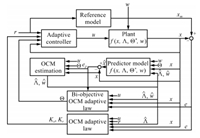
The adaptive control architecture with the bi-objective optimal control modification is presented in Fig. 1.

Proof. The optimal control modification adaptive laws (16) and (17) are called bi-objective because they use both the tracking error and the predictor error for adaptation and are derived from the following infinite-time horizon cost functions:

\begin{align} &J_{1}=\lim_{t_{f}\rightarrow\infty}\frac{1}{2}\int_{0}^{t_{f}} \left(e-\Delta_{1}\right)^{\rm T}Q\left(e-\Delta_{1}\right){\rm d}t, \end{align}

(23)

\begin{align} &J_{2}=\lim_{t_{f}\rightarrow\infty}\frac{1}{2}\int_{0}^{t_{f}} \left(e_{p}-\Delta_{2}\right)^{\rm T}R\left(e_{p}-\Delta_{2}\right){\rm d}t \end{align}

(24)

subject to (11) and (14),where $\Delta_{1}$ and $\Delta_{2}$ represent the unknown lower bounds of the tracking error and the predictor error,respectively.

The cost functions $J_{1}$ and $J_{2}$ are combined into the following bi-objective cost function:

\begin{align} J=J_{1}+J_{2}. \end{align}

(25)

The bi-objective cost function $J$ combines both the objectives of minimization of the tracking error and the predictor error bounded away from the origin. Geometrically,it represents a distance measured from a point on the trajectory of $e\left(t\right)$ and $e_{p}\left(t\right)$ to the normal surface of a hypersphere $B_{\Delta}=\left\{ e\left(t\right)\in {\bf R}^{n},e_{p}\left(t\right)\in{\bf R}^{n}:\frac{1}{2}\left(e-\Delta_{1}\right)^{\rm T}Q \left(e-\Delta_{1}\right)+\right.\left.\frac{1}{2}\left(e_{p}-\Delta_{2}\right)^{\rm T}R\left(e_{p}-\Delta_{2}\right) \le\Delta^{2}\right\} \subset\mathcal{D}\subset{\bf R}^{n}$ where $\Delta$ is the largest norm of the cost function $J$. The bi-objective cost function is designed to provide robustness by not seeking asymptotic tracking, but rather bounded tracking. By not requiring asymptotic tracking, the adaptation can be made more robust. Therefore,in effect,this framework provides a trade-off between performance and robustness by a suitable selection of the modification parameters $\nu$ and $\eta$ which influence the lower bounds $\Delta_{1}$ and $\Delta_{2}$. Better performance can be obtained by choosing small values of $\nu$ and/or $\eta$,but this decreases robustness of the adaptive laws to unmodeled dynamics,and vice versa.

The derivation of the bi-objective optimal control modification adaptive laws (16) $\sim$ (20) is established by the Pontryagin$'$s minimum principle. Using the optimal control framework,the Hamiltonian of the cost function is defined as

\begin{align} &H\!=\!\frac{1}{2}\left(e-\Delta_{1}\right)^{\rm T}Q\left(e-\Delta_{1}\right)+ \frac{1}{2}\left(e_{p}-\Delta_{2}\right)^{\rm T}R\left(e_{p}\!-\!\Delta_{2}\right)\!+\!\notag\\ &\quad\lambda^{\rm T}\left\{ A_{m}e+B\hat{\Lambda}\left[-\tilde{K}_{x}x- \tilde{K}_{r}r+\tilde{\Theta}^{\rm T}\Phi\left(x\right)\right]-w+B\epsilon\right\} \!+\!\notag\\ &\quad \mu^{\rm T}\Bigl\{ A_{m}e_{p}+B\tilde{\Lambda}\left[u+\Theta^{\rm T}\Phi\left(x\right)\right] +B\hat{\Lambda}\tilde{\Theta}^{\rm T}\Phi\left(x\right)+\notag\\ &\quad \tilde{w}+B\epsilon_{p}\Bigr\},\label{eq:-3-1} \end{align}

(26)

where $\lambda\left(t\right):\left[0,\infty\right)\rightarrow{\bf R}^{n}$ and $\mu\left(t\right):\left[0,\infty\right)\rightarrow{\bf R}^{n}$ are the adjoint variables or co-state vectors of $e\left(t\right)$ and $e_{p}\left(t\right)$,respectively.

The adjoint equations can be obtained from the necessary conditions of optimality as follows:

\begin{align} &\dot{\lambda}=-\nabla H_{e}^{\rm T}=-Q\left(e-\Delta_{1}\right)-A_{m}^{\rm T}\lambda,\label{eq:-4-1} \end{align}

(27)

\begin{align} &\dot{\mu}=-\nabla H_{e_{p}}^{\rm T}=-R\left(e_{p}-\Delta_{2}\right)-A_{m}^{\rm T}\mu, \end{align}

(28)

subject to the transversality conditions $\lambda\left(t_{f}\rightarrow\infty\right)=0$ and $\mu\left(t_{f}\rightarrow\infty\right)=0$ since both $e\left(0\right)$ and $e_{p}\left(0\right)$ are assumed to be known.

Treating $\tilde{K}_{x}\left(t\right)$, $\tilde{K}_{r}\left(t\right)$,$\tilde{\Theta}\left(t\right)$, $\tilde{\Lambda}\left(t\right)$,and $\hat{w}\left(t\right)$ as control variables,then the optimal control solutions are obtained by the following gradient-based adaptive laws:

\begin{align} &\dot{K}_{x}^{\rm T}=\dot{\tilde{K}}_{x}^{\rm T}=-\Gamma_{x}\nabla H_{\tilde{K}_{x}}=\Gamma_{x}x\lambda^{\rm T}B\hat{\Lambda},\label{eq:-6-1} \end{align}

(29)

\begin{align} &\dot{K}_{r}^{\rm T}=\dot{\tilde{K}}_{r}^{\rm T}=-\Gamma_{r}\nabla H_{\tilde{K}_{r}}=\Gamma_{r}r\lambda^{\rm T}B\hat{\Lambda},\label{eq:-7-1} \end{align}

(30)

\begin{align} &\dot{\Theta}=\dot{\tilde{\Theta}}=-\Gamma_{\Theta}\nabla H_{\tilde{\Theta}}^{\rm T}=-\Gamma_{\Theta}\Phi\left(x\right)\left(\lambda^{\rm T}+\mu^{\rm T}\right)B\hat{\Lambda},\label{eq:-5-1} \end{align}

(31)

\begin{align} &\dot{\hat{\Lambda}}^{\rm T}=\dot{\tilde{\Lambda}}^{\rm T}=-\Gamma_{\Lambda}\nabla H_{\tilde{\Lambda}}=-\Gamma_{\Lambda}\left[u+\Theta^{\rm T}\Phi\left(x\right)\right]\mu^{\rm T}B,\label{eq:-19-1} \end{align}

(32)

\begin{align} &\dot{\hat{w}}^{\rm T}=-\gamma_{w}\nabla H_{\hat{w}}=-\gamma_{w}\mu^{\rm T}.\label{eq:-348} \end{align}

(33)

The closed-form solutions can be obtained by eliminating the adjoint variables $\lambda\left(t\right)$ and $\mu\left(t\right)$ using the "sweep" method^[26] with the following assumed solutions of the adjoint equations

\begin{align} &\lambda=Pe+S\left[-K_{x}x-K_{r}r+\Theta^{\rm T}\Phi\left(x\right)\right],\label{eq:-8-1} \end{align}

(34)

\begin{align} &\mu=We_{p}+T\left[u+2\Theta^{\rm T}\Phi\left(x\right)\right]+V.\label{eq:-9-1} \end{align}

(35)

Substituting the adjoint solutions back into the adjoint equations yields

\begin{align} &\dot{P}e+PA_{m}e+PB\hat{\Lambda}\left[-K_{x}x-K_{r}r+\Theta^{\rm T}\Phi\left(x\right)\right]-\notag\\ &\qquad PB\hat{\Lambda}\left[-K_{x}^{*}x-K_{r}^{*}r+\Theta^{*{\rm T}}\Phi\left(x\right)\right]-Pw+PB\epsilon+\notag\\ &\qquad \dot{S}\left[-K_{x}x-K_{r}r+\Theta^{\rm T}\Phi\left(x\right)\right]+\notag\\ &\qquad S\frac{d\left[-K_{x}x-K_{r}r+\Theta^{\rm T}\Phi\left(x\right)\right]}{dt}=-Q\left(e-\Delta_{1}\right)-\notag\\ &\qquad A_{m}^{\rm T}Pe-A_{m}^{\rm T}S\left[-K_{x}x-K_{r}r+\Theta^{\rm T}\Phi\left(x\right)\right],\label{eq:-10-1} \end{align}

(36)

\begin{align} &\dot{W}e_{p}+WA_{m}e_{p}+WB\hat{\Lambda}\left[u+\Theta^{\rm T}\Phi\left(x\right)\right]-WB\Lambda\times\notag\\ &\qquad \left[u+\Theta^{\rm T}\Phi\left(x\right)\right]+WB\hat{\Lambda}\Theta^{\rm T}\Phi\left(x\right)-WB\hat{\Lambda}\Theta^{*{\rm T}}\Phi\left(x\right)+\notag\\ &\qquad W\hat{w}-Ww+WB\epsilon_{p}+\dot{T}\left[u+2\Theta^{\rm T}\Phi\left(x\right)\right]+\notag\\ &\qquad T\frac{{\rm d}\left[u+2\Theta^{\rm T}\Phi\left(x\right)\right]}{{\rm d}t}+\dot{V}=-R\left(e_{p}-\Delta_{2}\right)-\notag\\ &\qquad A_{m}^{\rm T}We_{p}-A_{m}^{\rm T}T\left[u+2\Theta^{\rm T}\Phi\left(x\right)\right]-A_{m}^{\rm T}V.\label{eq:-11-1} \end{align}

(37)

Equating terms yields the following equations:

\begin{align} &\dot{P}+PA_{m}+A_{m}^{\rm T}P+Q=0,\label{eq:-12-1} \end{align}

(38)

\begin{align} &\dot{S}+A_{m}^{\rm T}S+PB\hat{\Lambda}=0,\label{eq:-13-2} \end{align}

(39)

\begin{align} &Q\Delta_{1}+PB\hat{\Lambda}\left[-K_{x}^{*}x-K_{r}^{*}r+\Theta^{*{\rm T}}\Phi\left(x\right)\right]+Pw-\notag\\ &\qquad PB\epsilon-S\frac{{\rm d}\left[-K_{x}x-K_{r}r+\Theta^{\rm T}\Phi\left(x\right)\right]}{{\rm d}t}=0\label{eq:-23-1} \end{align}

(40)

\begin{align} &\dot{W}+WA_{m}+A_{m}^{\rm T}W+R=0\label{eq:-14-1} \end{align}

(41)

\begin{align} &\dot{T}+A_{m}^{\rm T}T+WB\hat{\Lambda}=0\label{eq:-15-1} \end{align}

(42)

\begin{align} &\dot{V}+A_{m}^{\rm T}V+W\hat{w}=0\label{eq:-364} \end{align}

(43)

\begin{align} &R\Delta_{2}+WB\Lambda\left[u+\Theta^{\rm T}\Phi\left(x\right)\right]+WB\hat{\Lambda}\Theta^{*{\rm T}}\Phi\left(x\right)+Ww-\notag\\ &\qquad WB\epsilon_{p}-T\frac{{\rm d}\left[u+2\Theta^{\rm T}\Phi\left(x\right)\right]}{{\rm d}t}=0, \end{align}

(44)

subject to the transversality conditions $P\left(t_{f}\rightarrow\infty\right)=0$, $S\left(t_{f}\rightarrow\infty\right)=0$, $W\left(t_{f}\rightarrow\infty\right)=0$,and $T\left(t_{f}\rightarrow\infty\right)=0$.

The existence and uniqueness of the solution of the Lyapunov differential equations are well-established^[27]. The infinite-time horizon solutions of the Lyapunov differential equations tend to their equilibrium solutions at $t=0$ as $\dot{P}\left(t\right)\rightarrow0$ and $\dot{W}\left(t\right)\rightarrow0$. Thus

\begin{align} &PA_{m}+A_{m}^{\rm T}P+Q=0,\label{eq:-12-1-1} \end{align}

(45)

\begin{align} &WA_{m}+A_{m}^{\rm T}W+R=0.\label{eq:-14-1-1} \end{align}

(46)

The solutions of $S\left(t\right)$,$T\left(t\right)$,and $V\left(t\right)$ also tend to their equilibrium solutions

\begin{align} &A_{m}^{\rm T}S+PB\hat{\Lambda}=0,\label{eq:-13-2-1} \end{align}

(47)

\begin{align} &A_{m}^{\rm T}T+WB\hat{\Lambda}=0,\label{eq:-15-1-1} \end{align}

(48)

\begin{align} &A_{m}^{\rm T}V+W\hat{w}=0.\label{eq:-364-1} \end{align}

(49)

As with any control design,performance and robustness are often considered as the two competing design requirements. Increasing robustness tends to require a compromise in performance and vice versa. Thus,to enable the bi-objective optimal control modification adaptive laws to be sufficiently flexible for control design,the modification parameters $\nu>0$ and $\eta>0$ are introduced as free design parameters to allow for adjustments of the bi-objective optimal control modification terms in the adaptive laws.

Thus,the solutions of $S\left(t\right)$,$T\left(t\right)$,and $V\left(t\right)$ are modified as

\begin{align} &S=-\nu A_{m}^{-{\rm T}}PB\hat{\Lambda},\label{eq:-24-1} \end{align}

(50)

\begin{align} &T=-\eta A_{m}^{-{\rm T}}WB\hat{\Lambda}, \end{align}

(51)

\begin{align} &V=-\eta A_{m}^{-{\rm T}}W\hat{w}.\label{eq:-365} \end{align}

(52)

Using the expression of $u\left(t\right)$,the adjoint solutions are then obtained as

\begin{align} &\lambda=Pe+\nu A_{m}^{-{\rm T}}PB\hat{\Lambda}u,\label{eq:-25-1} \end{align}

(53)

\begin{align} &\mu=We_{p}-\eta A_{m}^{-{\rm T}}W\left\{ B\hat{\Lambda}\left[u+2\Theta^{\rm T}\Phi\left(x\right)\right]+\hat{w}\right\}. \end{align}

(54)

Substituting the adjoint solutions into the gradient-based adaptive laws yields the bi-objective optimal control modification adaptive laws (16) $\sim$ (20).

The bounds on $\Delta_{1}\left(t\right)$ and $\Delta_{2}\left(t\right)$ as $t_{f}\rightarrow\infty$ are then given by

\begin{align} &\left\Vert \Delta_{1}\right\Vert \le\frac{1}{\lambda_{\rm min}\left(Q\right)}\Biggl [\left\Vert PB\hat{\Lambda}\right\Vert \left\Vert -K_{x}^{*}x-\Delta K_{r}^{*}r+ \Theta^{*{\rm T}}\Phi\left(x\right)\right\Vert+ \notag\\ &\qquad \lambda_{\rm max}\left(P\right)w_{0}+\left\Vert PB\right\Vert \epsilon_{0}+\notag\\ &\qquad \nu\left\Vert A_{m}^{-{\rm T}}PB\hat{\Lambda}\right\Vert \left\Vert \frac{{\rm d}\left[-K_{x}x-K_{r}r+\Theta^{\rm T}\Phi\left(x\right)\right]}{{\rm d}t}\right\Vert \Biggr], \end{align}

(55)

\begin{align} &\left\Vert \Delta_{2}\right\Vert \le\frac{1}{\lambda_{\rm min}\left(R\right)}\Biggl [\left\Vert WB\Lambda\right\Vert \left\Vert u+\Theta^{\rm T}\Phi\left(x\right)\right\Vert +\notag\\ &\qquad \left\Vert WB\hat{\Lambda}\right\Vert \left\Vert \Theta^{*{\rm T}}\Phi\left(x\right) \right\Vert +\lambda_{\rm max}\left(W\right)w_{0}+\left\Vert WB\right\Vert \epsilon_{p_{0}}+\notag\\ &\qquad \eta\left\Vert A_{m}^{-{\rm T}}WB\hat{\Lambda}\right\Vert \left\Vert \frac{{\rm d}\left[u+\Theta^{\rm T}\Phi\left(x\right)\right]}{{\rm d}t}\right\Vert \Biggr], \end{align}

(56)

which are dependent upon the modification parameters,control effectiveness uncertainty,matched uncertainty,unmatched disturbance,and residual tracking error and predictor error.

Note that if $R=Q$ and $\eta=\nu$,then the bi-objective optimal control modification adaptive laws for $\Theta\left(t\right)$, $\hat{\Lambda}\left(t\right)$,and $\hat{w}\left(t\right)$ become

\begin{align} \dot{\Theta}=-\Gamma_{\Theta}\Phi\left(x\right)\left(e^{\rm T}P+e_{p}^{\rm T}P\right.-\\ \left.\nu\left\{ 2\Phi^{\rm T}\left(x\right)\Theta\hat{\Lambda}^{\rm T}B^{\rm T}+\hat{w}^{\rm T}\right\} PA_{m}^{-1}\right)B\hat{\Lambda},\label{eq:-20-1} \end{align}

(57)

\begin{align} \dot{\hat{\Lambda}}^{\rm T}=-\Gamma_{\Lambda}\left[u+\Theta^{\rm T}\Phi\left(x\right)\right]\left(e_{p}^{\rm T}P\right.-\\ \left.\nu\left\{ \left[u+2\Theta^{\rm T}\Phi\left(x\right)\right]^{\rm T}\hat{\Lambda}^{\rm T}B^{\rm T}+\hat{w}^{\rm T}\right\} PA_{m}^{-1}\right)B,\label{eq:-20-1-1} \end{align}

(58)

\begin{align} \dot{\hat{w}}^{\rm T}=-\gamma_{w}\left(e_{p}^{\rm T}P\right.-\\ \left.\nu\left\{ \left[u+2\Theta^{\rm T}\Phi\left(x\right)\right]^{\rm T}\hat{\Lambda}^{\rm T}B^{\rm T}+\hat{w}^{\rm T}\right\} PA_{m}^{-1}\right).\label{eq:-363-2} \end{align}

(59)

Theorem. The bi-objective optimal control modification adaptive laws (16) $\sim$ (20) result in stable and uniformly ultimately bounded tracking error $e\left(t\right)$ and bounded predictor error $e_{p}\left(t\right)$.

Proof. Choose a Lyapunov candidate function

\begin{align} &V=e^{\rm T}Pe+e_{p}^{\rm T}We_{p}+\textrm{trace}\left(\tilde{K}_{x}\Gamma_{x}^{-1}\tilde{K}_{x}^{\rm T}\right)+\notag\\ &\qquad \textrm{trace}\left(\tilde{K}_{r}\Gamma_{r}^{-1}\tilde{K}_{r}^{\rm T}\right)+\textrm{trace}\left(\tilde{\Theta}^{\rm T}\Gamma_{\Theta}^{-1}\tilde{\Theta}\right)+\notag\\ &\qquad \textrm{trace}\left(\tilde{\Lambda}\Gamma_{\Lambda}^{-1}\tilde{\Lambda}^{\rm T}\right)+\tilde{w}^{\rm T}\gamma_{w}^{-1}\tilde{w}.\label{DUPLICATE: eq:-349} \end{align}

(60)

Evaluating $\dot{V}\left(e,e_{p},\tilde{K}_{x},\tilde{K}_{r},\tilde{\Theta},\tilde{\Lambda},\tilde{w}\right)$ yields

\begin{align} &\dot{V}=-e^{\rm T}Qe+2e^{\rm T}PB\hat{\Lambda}\left[-\tilde{K}_{x}x-\tilde{K}_{r}r+\tilde{\Theta}^{\rm T}\Phi\left(x\right)\right]-\notag\\ &\qquad 2e^{\rm T}Pw+2e^{\rm T}PB\epsilon-e_{p}^{\rm T}Re_{p}+\notag\\ &\qquad 2e_{p}^{\rm T}WB\left\{ \tilde{\Lambda}\left[u+\Theta^{\rm T}\Phi\left(x\right)\right]+\hat{\Lambda}\tilde{\Theta}^{\rm T}\Phi\left(x\right)\right\}+\notag \\ &\qquad 2e_{p}^{\rm T}WB\epsilon_{p}-2\dot{w}^{\rm T}\gamma_{w}^{-1}\tilde{w}+\notag\\ &\qquad 2\textrm{trace}\left(\tilde{K}_{x}x\left(e^{\rm T}P+\nu u^{\rm T}\hat{\Lambda}^{\rm T}B^{\rm T}PA_{m}^{-1}\right)B\hat{\Lambda}\right)+\notag\\ &\qquad 2\textrm{trace}\left(\tilde{K}_{r}r\left(e^{\rm T}P+\nu u^{\rm T}\hat{\Lambda}^{\rm T}B^{\rm T}PA_{m}^{-1}\right)B\hat{\Lambda}\right)-\notag\\ &\qquad 2\textrm{trace}\Biggl(\tilde{\Theta}^{\rm T}\Phi\left(x\right)\biggl(e^{\rm T}P+\nu u^{\rm T}\hat{\Lambda}^{\rm T}B^{\rm T}PA_{m}^{-1}+e_{p}^{\rm T}W-\notag\\ &\qquad \eta\left\{ \left[u+2\Theta^{\rm T}\Phi\left(x\right)\right]^{\rm T}\hat{\Lambda}^{\rm T}B^{\rm T}+\hat{w}^{\rm T}\right\} WA_{m}^{-1}\biggr)B\hat{\Lambda}\Biggr)-\notag\\ &\qquad 2\textrm{trace}\Biggl(\tilde{\Lambda}\left[u+\Theta^{\rm T}\Phi\left(x\right)\right]\biggl(e_{p}^{\rm T}W-\notag\\ &\qquad \eta\left\{ \left[u+2\Theta^{\rm T}\Phi\left(x\right)\right]^{\rm T}\hat{\Lambda}^{\rm T}B^{\rm T}+\hat{w}^{\rm T}\right\} WA_{m}^{-1}\biggr)B\Biggr)+\notag\\ &\qquad 2\left(\eta\left\{ \left[u+2\Theta^{\rm T}\Phi\left(x\right)\right]^{\rm T}\hat{\Lambda}^{\rm T}B^{\rm T}+\hat{w}^{\rm T}\right\} WA_{m}^{-1}\right)\tilde{w}. \end{align}

(61)

Using the trace identity $\textrm{trace}\left(C^{\rm T}D\right)=DC^{\rm T}$ where $C$ and $D$ are any arbitrary vectors of the same dimension, $\dot{V}\left(e,e_{p},\tilde{K}_{x},\tilde{K}_{r},\tilde{\Theta},\tilde{\Lambda},\tilde{w}\right)$ can be further simplified as

\begin{align} &\dot{V}=-e^{\rm T}Qe-2e^{\rm T}Pw+2e^{\rm T}PB\epsilon-e_{p}^{\rm T}Re_{p}+2e_{p}^{\rm T}WB\epsilon_{p}-\notag\\ &\qquad 2\dot{w}^{\rm T}\gamma_{w}^{-1}\tilde{w}+2\nu u^{\rm T}\hat{\Lambda}^{\rm T}B^{\rm T}PA_{m}^{-1}B\hat{\Lambda}\tilde{u}+\notag\\ &\qquad 2\eta\textrm{trace}\biggl(\tilde{\Theta}^{\rm T}\Phi\left(x\right)\times\notag\\ &\qquad \left\{ \left[u+2\Theta^{\rm T}\Phi\left(x\right)\right]^{\rm T}\hat{\Lambda}^{\rm T}B^{\rm T}+\hat{w}^{\rm T}\right\} WA_{m}^{-1}B\hat{\Lambda}\biggr)+\notag\\ &\qquad 2\eta\textrm{trace}\biggl(\tilde{\Lambda}\left[u+\Theta^{\rm T}\Phi\left(x\right)\right]\times\notag\\ &\qquad \left\{ \left[u+2\Theta^{\rm T}\Phi\left(x\right)\right]^{\rm T}\hat{\Lambda}^{\rm T}B^{\rm T}+\hat{w}^{\rm T}\right\} WA_{m}^{-1}B\biggr)+\notag\\ &\qquad 2\eta\textrm{trace}\biggl(\tilde{w}\times\notag\\ &\qquad \left\{ \left[u+2\Theta^{\rm T}\Phi\left(x\right)\right]^{\rm T}\hat{\Lambda}^{\rm T}B^{\rm T}+\hat{w}^{\rm T}\right\} WA_{m}^{-1}\biggr), \end{align}

(62)

where $\tilde{u}=\tilde{K}_{x}x+\tilde{K}_{r}r-\tilde{\Theta}^{\rm T}\Phi\left(x\right)$.

Let $\bar{B}=\left[\begin{array}{ccc} B\hat{\Lambda} & B & I\end{array}\right]\in{\bf R}^{n\times\left(2m+n\right)}$, $\Omega=\left[\begin{array}{ccc} \Theta & 0 & 0\\ 0 & \hat{\Lambda}^{\rm T} & 0\\ 0 & 0 & \hat{w}^{\rm T} \end{array}\right]\in{\bf R}^{\left(p+m+1\right)\times\left(2m+n\right)}$, $\Psi\left(x,r\right)=\left[\begin{array}{c} \Phi\left(x\right)\\ u+\Theta^{\rm T}\Phi\left(x\right)\\ 1 \end{array}\right]\in{\bf R}^{p+m+1}$. Then

\begin{align} &\textrm{trace}\left(\tilde{\Omega}^{\rm T}\Psi\left(x,r\right)\Psi^{\rm T}\left(x,r\right)\Omega\bar{B}^{\rm T}WA_{m}^{-1}\bar{B}\right)=\notag\\ &\textrm{trace}\biggl(\tilde{\Theta}^{\rm T}\Phi\left(x\right)\times\notag\\ &\qquad \left\{ \left[u+2\Theta^{\rm T}\Phi\left(x\right)\right]^{\rm T}\hat{\Lambda}^{\rm T}B^{\rm T}+\hat{w}^{\rm T}\right\} WA_{m}^{-1}B\hat{\Lambda}\biggr)+\notag\\ &\qquad \textrm{trace}\biggl(\tilde{\Lambda}\left[u+\Theta^{\rm T}\Phi\left(x\right)\right]\times\notag\\ &\qquad \left\{ \left[u+2\Theta^{\rm T}\Phi\left(x\right)\right]^{\rm T}\hat{\Lambda}^{\rm T}B^{\rm T}+\hat{w}^{\rm T}\right\} WA_{m}^{-1}B\biggr)+\notag\\ &\qquad \textrm{trace}\biggl(\tilde{w}\times\notag\\ &\qquad \left\{ \left[u+2\Theta^{\rm T}\Phi\left(x\right)\right]^{\rm T}\hat{\Lambda}^{\rm T}B^{\rm T}+\hat{w}^{\rm T}\right\} WA_{m}^{-1}\biggr), \end{align}

(63)

where $\tilde{\Omega}=\Omega-\Omega^{*}$ and $\Omega^{*}=\left[\begin{array}{ccc} \Theta^{*} & 0 & 0\\ 0 & \Lambda^{\rm T} & 0\\ 0 & 0 & w^{\rm T} \end{array}\right]\in{\bf R}^{\left(p+m+1\right)\times\left(2m+n\right)}$.

Thus,

\begin{align} &\dot{V}=-e^{\rm T}Qe-2e^{\rm T}Pw+2e^{\rm T}PB\epsilon-e_{p}^{\rm T}Re_{p}+2e_{p}^{\rm T}WB\epsilon_{p}-\notag\\ &\qquad2\dot{w}^{\rm T}\gamma_{w}^{-1}\tilde{w}+2\nu u^{\rm T}\hat{\Lambda}^{\rm T}B^{\rm T}PA_{m}^{-1}B\hat{\Lambda}\tilde{u}+\notag\\ &\qquad2\eta\Psi^{\rm T}\left(x,r\right)\Omega\bar{B}^{\rm T}WA_{m}^{-1}\bar{B}\tilde{\Omega}^{\rm T}\Psi\left(x,r\right). \end{align}

(64)

Note that $B^{\rm T}PA_{m}^{-1}B^{\rm T}$ and $\bar{B}^{\rm T}WA_{m}^{-1}\bar{B}$ are both negative-definite matrices, therefore

\begin{align} &\dot{V}=-e^{\rm T}Qe-2e^{\rm T}Pw+2e^{\rm T}PB\epsilon-e_{p}^{\rm T}Re_{p}+2e_{p}^{\rm T}WB\epsilon_{p}-\notag\\ &\qquad 2\dot{w}^{\rm T}\gamma_{w}^{-1}\tilde{w}-\nu\tilde{u}^{\rm T}\hat{\Lambda}^{\rm T}B^{\rm T}A_{m}^{-{\rm T}}QA_{m}^{-1}B\hat{\Lambda}\tilde{u}-\notag\\ &\qquad \eta\Psi^{\rm T}\left(x,r\right)\tilde{\Omega}\bar{B}^{\rm T}A_{m}^{-{\rm T}}RA_{m}^{-1}\bar{B}\tilde{\Omega}^{\rm T}\Psi\left(x,r\right)+\notag\\ &\qquad 2\nu u^{*{\rm T}}\hat{\Lambda}^{\rm T}B^{\rm T}PA_{m}^{-1}B\hat{\Lambda}\tilde{u}+\notag\\ &\qquad 2\eta\Psi^{\rm T}\left(x,r\right)\Omega^{*}\bar{B}^{\rm T}WA_{m}^{-1}\bar{B}\tilde{\Omega}^{\rm T}\Psi\left(x,r\right). \end{align}

(65)

Let $K=\left[\begin{array}{ccc} K_{x} & K_{r} & -\Theta^{\rm T}\end{array}\right]\in{\bf R}^{m\times\left(n+r+p\right)}$,and $z\left(x,r\right)=\left[\begin{array}{c} x\\ r\\ \Phi\left(x\right) \end{array}\right]\in{\bf R}^{n+r+p}$. Then $u=Kz\left(x,r\right)$ and

\begin{align} &\dot{V}\le-\lambda_{\rm min}\left(Q\right)\left\Vert e\right\Vert ^{2}+2\left\Vert e\right\Vert \lambda_{\rm max} \left(P\right)w_{0}+2\left\Vert e\right\Vert \left\Vert PB\right\Vert \epsilon_{0}-\notag\\ &\qquad \lambda_{\rm min}\left(R\right)\left\Vert e_{p}\right\Vert ^{2}+2\left\Vert e_{p}\right\Vert \left\Vert WB\right\Vert \epsilon_{p_{0}}+2\gamma_{w}^{-1}\left\Vert \tilde{\Omega}\right\Vert \delta_{0}-\notag\\ &\qquad \nu\lambda_{\rm min}\left(B^{\rm T}A_{m}^{-{\rm T}}QA_{m}^{-1}B\right)\left\Vert z\left(x,r\right)\right\Vert ^{2} \left\Vert \hat{\Lambda}\right\Vert ^{2}\left\Vert \tilde{K}\right\Vert ^{2}+\notag\\ &\qquad 2\nu\left\Vert z\left(x,r\right)\right\Vert ^{2}\left\Vert B^{\rm T}PA_{m}^{-1}B\right\Vert \left\Vert \hat{\Lambda}\right\Vert ^{2}\left\Vert \tilde{K}\right\Vert K_{0}-\notag\\ &\qquad \eta\lambda_{\rm min}\left(A_{m}^{-{\rm T}}RA_{m}^{-1}\right)\left\Vert \Psi\left(x,r\right) \right\Vert ^{2}\left\Vert \bar{B}\right\Vert ^{2}\left\Vert \tilde{\Omega}\right\Vert ^{2}+\notag\\ &\qquad 2\eta\left\Vert WA_{m}^{-1}\right\Vert \left\Vert \Psi\left(x,r\right)\right\Vert ^{2}\left\Vert \bar{B}\right\Vert ^{2}\left\Vert \tilde{\Omega}\right\Vert \Omega_{0} \end{align}

(66)

where $K_{0}=\left\Vert K^{*}\right\Vert $ and $\Omega_{0}=\left\Vert \Omega^{*}\right\Vert $.

Let $c_{1}=\lambda_{\rm min}\left(Q\right)$,$c_{2}=\frac{\lambda_{\rm max}\left(P\right)w_{0}+\left\Vert PB\right\Vert \epsilon_{0}}{\lambda_{\rm min}\left(Q\right)}$,$c_{3}=\lambda_{\rm min}\left(R\right)$, $c_{4}=\frac{\left\Vert WB\right\Vert \epsilon_{p_{0}}}{\lambda_{\rm min}\left(R\right)}$, $c_{5}=\lambda_{\rm min}\left(B^{\rm T}A_{m}^{-{\rm T}}QA_{m}^{-1}B\right)\left\Vert z\left(x,r\right)\right\Vert ^{2}$, $c_{6}=\frac{\left\Vert B^{\rm T}PA_{m}^{-1}B\right\Vert K_{0}}{\lambda_{\rm min}\left(B^{\rm T}A_{m}^{-{\rm T}}QA_{m}^{-1}B\right)}$, $c_{7}=\lambda_{\rm min}\left(A_{m}^{-{\rm T}}RA_{m}^{-1}\right)\left\Vert \Psi\left(x,r\right)\right\Vert ^{2}$, and $c_{8}=\frac{\left\Vert WA_{m}^{-1}\right\Vert \Omega_{0}}{\lambda_{\rm min}\left(A_{m}^{-{\rm T}}RA_{m}^{-1}\right)}+\frac{\gamma_{w}^{-1}\delta_{0}}{\eta c_{7}\left\Vert \bar{B}\right\Vert ^{2}}$. Then

\begin{align} &\dot{V}\le-c_{1}\left(\left\Vert e\right\Vert -c_{2}\right)^{2}+c_{1}c_{2}^{2}-c_{3}\left(\left\Vert e_{p}\right\Vert -c_{4}\right)^{2}+c_{3}c_{4}^{2}-\notag\\ &\qquad \nu c_{5}\left\Vert \hat{\Lambda}\right\Vert ^{2}\left(\left\Vert \tilde{K}\right\Vert -c_{6}\right)^{2}+\nu c_{5}c_{6}^{2}\left\Vert \hat{\Lambda}\right\Vert ^{2}-\notag\\ &\qquad \eta c_{7}\left\Vert \bar{B}\right\Vert ^{2}\left(\left\Vert \tilde{\Omega}\right\Vert -c_{8}\right)^{2}+\eta c_{7}c_{8}^{2}\left\Vert \bar{B}\right\Vert ^{2}. \end{align}

(67)

Note that

\begin{align} \left\Vert \hat{\Lambda}\right\Vert \le\left\Vert \Omega\right\Vert \Rightarrow\left\Vert \tilde{\Lambda}\right\Vert \le\left\Vert \tilde{\Omega}\right\Vert,\label{eq:-2} \end{align}

(68)

\begin{align} &\left\Vert \hat{\Lambda}\right\Vert ^{2}=\left\Vert \Lambda+\tilde{\Lambda}\right\Vert ^{2}\le\left\Vert \Lambda\right\Vert ^{2}+2\left\Vert \Lambda\right\Vert \left\Vert \tilde{\Lambda}\right\Vert +\left\Vert \tilde{\Lambda}\right\Vert ^{2}\le\notag\\ &\qquad \left\Vert \Lambda\right\Vert ^{2}+2\left\Vert \Lambda\right\Vert \left\Vert \tilde{\Omega}\right\Vert +\left\Vert \tilde{\Omega}\right\Vert ^{2}, \end{align}

(69)

\begin{align} &\left\Vert \bar{B}\right\Vert ^{2}=\left\Vert \bar{B}^{*}+\tilde{B}\right\Vert ^{2}\le\left\Vert \bar{B}^{*}\right\Vert ^{2}+2\left\Vert \bar{B}^{*}\right\Vert \left\Vert \tilde{B}\right\Vert +\left\Vert \tilde{B}\right\Vert ^{2}\le\notag\\ &\qquad \left\Vert \bar{B}^{*}\right\Vert ^{2}+2\left\Vert \bar{B}^{*}\right\Vert \left\Vert B\right\Vert \left\Vert \tilde{\Lambda}\right\Vert +\left\Vert B\right\Vert ^{2}\left\Vert \tilde{\Lambda}\right\Vert ^{2}\le\notag\\ &\qquad\left\Vert \bar{B}^{*}\right\Vert ^{2}+2\left\Vert \bar{B}^{*}\right\Vert \left\Vert B\right\Vert \left\Vert \tilde{\Omega}\right\Vert +\left\Vert B\right\Vert ^{2}\left\Vert \tilde{\Omega}\right\Vert ^{2}, \end{align}

(70)

where $\tilde{B}=\bar{B}-\bar{B}^{*}$ and $\bar{B}^{*}=\left[\begin{array}{ccc} B\Lambda & B & I\end{array}\right]\in{\bf R}^{n\times\left(2m+n\right)}$.

Note that $\dot{V}\left(e,e_{p},\tilde{K},\tilde{\Omega}\right)$ can be upper-bounded by maximizing the terms in (66) that depend on $\left\Vert \hat{\Lambda}\right\Vert $ and $\left\Vert \bar{B}\right\Vert $ which in turn depend on $\left\Vert \tilde{K}\right\Vert $ and $\left\Vert \tilde{\Omega}\right\Vert $. Thus,taking the partial derivatives with respect to $\left\Vert \tilde{K}\right\Vert $ and $\left\Vert \tilde{\Omega}\right\Vert $ and setting them to zero yield $\left\Vert \tilde{K}\right\Vert =c_{6}$,and

\begin{align} &2\nu c_{5}c_{6}^{2}\left(\left\Vert \Lambda\right\Vert +\left\Vert \tilde{\Omega}\right\Vert \right)-2\eta c_{7}\left\Vert \bar{B}\right\Vert ^{2}\left(\left\Vert \tilde{\Omega}\right\Vert -c_{8}\right)-\notag\\ &\qquad2\eta c_{7}\left\Vert B\right\Vert \left\Vert \tilde{\Omega}\right\Vert \left(\left\Vert \bar{B}^{*}\right\Vert +\left\Vert B\right\Vert \left\Vert \tilde{\Omega}\right\Vert \right)\left(\left\Vert \tilde{\Omega}\right\Vert -2c_{8}\right)=\notag\\ &\qquad 0,\label{eq:-8} \end{align}

(71)

whose solution yields one of the roots $\left\Vert \tilde{\Omega}\right\Vert =c_{9}$ that maximizes these terms.

Consider two limiting cases:

1) When $\left\Vert \tilde{\Omega}\right\Vert \ll1$ and $\left\Vert \tilde{\Omega}\right\Vert \ll\left\Vert \Lambda\right\Vert $,then $\left\Vert \hat{\Lambda}\right\Vert ^{2}\le\left(1+\epsilon_{1}\right)^{2}\left\Vert \Lambda\right\Vert ^{2}$ and $\left\Vert \bar{B}\right\Vert ^{2}\le\left(1+\epsilon_{2}\right)^{2}\left\Vert \bar{B}^{*}\right\Vert ^{2}$ where $\epsilon_{1}=\frac{\left\Vert \tilde{\Omega}\right\Vert }{\left\Vert \Lambda\right\Vert }>0$ and $\epsilon_{2}=\frac{\left\Vert B\right\Vert \left\Vert \tilde{\Omega}\right\Vert }{\left\Vert \bar{B}^{*}\right\Vert }>0$ are small positive constants. Setting the partial derivative with respect to $\left\Vert \tilde{\Omega}\right\Vert $ to zero yields

\begin{align} -2\eta c_{7}\left(1+\epsilon_{2}\right)^{2}\left\Vert \bar{B}^{*}\right\Vert ^{2}\left(\left\Vert \tilde{\Omega}\right\Vert -c_{8}\right)=0\label{eq:-11} \end{align}

(72)

whose solution is $\left\Vert \tilde{\Omega}\right\Vert =c_{9}=c_{8}$ which maximizes the terms that depend on $\left\Vert \tilde{\Omega}\right\Vert $ since the second partial derivative with respect to $\left\Vert \tilde{\Omega}\right\Vert $ is always negative.

2) When $\left\Vert \tilde{\Omega}\right\Vert \gg1$ and $\left\Vert \tilde{\Omega}\right\Vert \gg\left\Vert \Lambda\right\Vert $,then $\left\Vert \hat{\Lambda}\right\Vert ^{2}\le\left(1+\epsilon_{3}\right)^{2}\left\Vert \tilde{\Omega}\right\Vert ^{2}$ and $\left\Vert \bar{B}\right\Vert ^{2}\le\left(1+\epsilon_{4}\right)^{2}\left\Vert B\right\Vert ^{2}\left\Vert \tilde{\Omega}\right\Vert ^{2}$ where $\epsilon_{3}=\frac{\left\Vert \Lambda\right\Vert }{\left\Vert \tilde{\Omega}\right\Vert }>0$ and $\epsilon_{4}=\frac{\left\Vert \bar{B}^{*}\right\Vert }{\left\Vert B\right\Vert \left\Vert \tilde{\Omega}\right\Vert }>0$ are small positive constants. Evaluating the partial derivative with respect to $\left\Vert \tilde{\Omega}\right\Vert $ gives

\begin{align} &2\nu c_{5}c_{6}^{2}\left(1+\epsilon_{3}\right)^{2}\left\Vert \tilde{\Omega}\right\Vert -4\eta c_{7}\left(1+\epsilon_{4}\right)^{2}\left\Vert B\right\Vert ^{2}\left\Vert \tilde{\Omega}\right\Vert ^{3}+\notag\\ &\qquad 6\eta c_{7}\left(1+\epsilon_{4}\right)^{2}\left\Vert B\right\Vert ^{2}\left\Vert \tilde{\Omega}\right\Vert ^{2}c_{8}=0, \end{align}

(73)

Equation (73) yields only one positive root $\left\Vert \tilde{\Omega}\right\Vert =c_{9}=\frac{3c_{8}}{4}\left(1+\sqrt{1+\frac{8\nu c_{5}c_{6}^{2}\left(1+\epsilon_{3}\right)^{2}}{9\eta c_{7}c_{8}^{2}\left(1+\epsilon_{4}\right)^{2}\left\Vert B\right\Vert ^{2}}}\right)$. Evaluating the second partial derivative with respect to $\left\Vert \tilde{\Omega}\right\Vert $ at this root gives a negative value of $-4\nu c_{5}c_{6}^{2}\left(1+\epsilon_{3}\right)^{2}-6\eta c_{7}c_{8}c_{9}\left(1+\epsilon_{4}\right)^{2}\left\Vert B\right\Vert ^{2}$. This shows that $\left\Vert \tilde{\Omega}\right\Vert =c_{9}$ maximizes the terms that depend on $\left\Vert \tilde{\Omega}\right\Vert $.

Therefore,this results in $\left\Vert \hat{\Lambda}\right\Vert ^{2}\le\Lambda_{0}^{2}:=\left\Vert \Lambda\right\Vert ^{2}+2\left\Vert \Lambda\right\Vert c_{9}+c_{9}^{2}$ and $\left\Vert \bar{B}\right\Vert ^{2}\le B_{0}^{2}:=\left\Vert \bar{B}^{*}\right\Vert ^{2}+2\left\Vert \bar{B}^{*}\right\Vert \left\Vert B\right\Vert c_{9}+\left\Vert B\right\Vert ^{2}c_{9}^{2}$. Thus, $\dot{V}\left(e,e_{p},\tilde{K},\tilde{\Omega}\right)\le0$ outside a compact set $\mathcal{S}$ defined as

\begin{align} &\mathcal{S}=\Biggl\{\left(e\left(t\right),e_{p}\left(t\right),\tilde{K}\left(t\right),\tilde{\Omega}\left(t\right)\right):c_{1}\left(\left\Vert e\right\Vert -c_{2}\right)^{2}+\notag\\ &\qquad c_{3}\left(\left\Vert e_{p}\right\Vert -c_{4}\right)^{2}+\nu c_{5}\Lambda_{0}^{2}\left(\left\Vert \tilde{K}\right\Vert -c_{6}\right)^{2}+\notag\\ &\qquad \eta c_{7}B_{0}^{2}\left(\left\Vert \tilde{\Omega}\right\Vert -c_{8}\right)^{2}\le c_{1}c_{2}^{2}+c_{3}c_{4}^{2}+\notag\\ &\qquad \nu c_{5}c_{6}^{2}\Lambda_{0}^{2}+\eta c_{7}c_{8}^{2}B_{0}^{2}\Biggr\}. \end{align}

(74)

This implies

\begin{align} &\left\Vert e\right\Vert \ge c_{2}+\sqrt{c_{2}^{2}+\frac{c_{3}c_{4}^{2}+\nu c_{5}c_{6}^{2}\Lambda_{0}^{2}+\eta c_{7}c_{8}^{2}B_{0}^{2}}{c_{1}}}=r, \end{align}

(75)

\begin{align} &\left\Vert e_{p}\right\Vert \ge c_{4}+\sqrt{c_{4}^{2}+\frac{c_{1}c_{2}^{2}+\nu c_{5}c_{6}^{2}\Lambda_{0}^{2}+\eta c_{7}c_{8}^{2}B_{0}^{2}}{c_{3}}}=p, \end{align}

(76)

\begin{align} &\left\Vert \tilde{K}\right\Vert \ge c_{6}+\sqrt{c_{6}^{2}+\frac{c_{1}c_{2}^{2}+c_{3}c_{4}^{2}+\eta c_{7}c_{8}^{2}B_{0}^{2}}{\nu c_{5}\Lambda_{0}^{2}}}=\alpha, \end{align}

(77)

\begin{align} \left\Vert \tilde{\Omega}\right\Vert \ge c_{8}+\sqrt{c_{8}^{2}+\frac{c_{1}c_{2}^{2}+c_{3}c_{4}^{2}+\nu c_{5}c_{6}^{2}\Lambda_{0}^{2}}{\eta c_{7}B_{0}^{2}}}=\beta,\label{eq:-362} \end{align}

(78)

There exist $z_{0}$ and $\Psi_{0}$ such that $\left\Vert z\left(x,r\right)\right\Vert \le z_{0}$ and $\left\Vert \Psi\left(x,r\right)\right\Vert \le\Psi_{0}$ for any $0 < \nu < \nu_{\rm max}$ and $0 < \eta < \eta_{\rm max}$ that satisfy the following inequalities:

\begin{align} &\varphi\left(\left\Vert x\right\Vert ,\left\Vert x_{m}\right\Vert ,Q, \nu,w_{0},\epsilon_{0},\Lambda_{0},K_{0}\right)=-c_{1}\left\Vert x\right\Vert ^{2}+\notag\\ &\qquad 2\left(c_{1}c_{2}+\lambda_{\rm max}\left(Q\right)\left\Vert x_{m}\right\Vert \right)\left\Vert x\right\Vert +2c_{1}c_{2}\left\Vert x_{m}\right\Vert- \notag\\ &\qquad c_{1}\left\Vert x_{m}\right\Vert ^{2}+c_{3}c_{4}^{2}+\nu c_{5}\left(\left\Vert z\left(x,r\right)\right\Vert \right)c_{6}^{2}\Lambda_{0}^{2}+\notag\\ &\qquad \eta c_{7}\left(\left\Vert \Psi\left(x,r\right)\right\Vert \right)c_{8}^{2}B_{0}^{2}\le0,\label{eq:-196-3} \end{align}

(79)

\begin{align} &\phi\left(\left\Vert x_{p}\right\Vert ,\left\Vert x_{m}\right\Vert ,R,\eta,\dot{w}_{0}, \epsilon_{p_{0}},B_{0},\Omega_{0}\right)=-c_{3}\left\Vert x_{p}\right\Vert ^{2}+\notag\\ &\qquad 2\left(c_{3}c_{4}+\lambda_{\rm max}\left(R\right)\left\Vert x\right\Vert \right) \left\Vert x_{p}\right\Vert +2c_{3}c_{4}\left\Vert x\right\Vert -c_{3}\left\Vert x\right\Vert ^{2}+\notag\\ &\qquad c_{1}c_{2}^{2}+\nu c_{5}\left(\left\Vert z\left(x,r\right)\right\Vert \right)c_{6}^{2}\Lambda_{0}^{2}+\notag\\ &\qquad \eta c_{7}\left(\left\Vert \Psi\left(x,r\right)\right\Vert \right)c_{8}^{2}B_{0}^{2}\le0.\label{eq:-196-3-1} \end{align}

(80)

Then,the lower bounds which are dependent on $\left\Vert z\left(x,r\right)\right\Vert $ and $\left\Vert \Psi\left(x,r\right)\right\Vert $ also exist. Since $\dot{V}\left(e,e_{p},\tilde{K},\tilde{\Omega}\right)\le0$ outside the compact set $\mathcal{S}$, $\lim_{t\rightarrow\infty}V\left(e,e_{p},\tilde{K},\tilde{\Omega}\right)\le V_{0}$,where $V_{0}$ is the largest lower bound of $V\left(e,e_{p},\tilde{K},\tilde{\Omega}\right)$ which is given by

\begin{align} &V_{0}=\lambda_{\rm max}\left(P\right)r^{2}+\lambda_{\rm max}\left(W\right)p^{2}+\lambda_{\rm max} \left(\Gamma_{x}^{-1}\right)\alpha^{2}+\notag\\ &\qquad \lambda_{\rm max}\left(\Gamma_{r}^{-1}\right)\alpha^{2}+\lambda_{\rm max}\left(\Gamma_{\Theta}^{-1}\right) \left(\alpha^{2}+\beta^{2}\right)+\notag\\ &\qquad \lambda_{\rm max}\left(\Gamma_{\Lambda}^{-1}\right)\beta^{2}+\gamma_{w}^{-1}\beta^{2}.\label{eq:-16} \end{align}

(81)

Then

\begin{align} &\lambda_{\rm min}\left(P\right)\lim_{t\rightarrow\infty}\left\Vert e\right\Vert ^{2}\le\lim_{t\rightarrow\infty}V\left(e,e_{p},\tilde{K},\tilde{\Omega}\right)\le V_{0},\label{eq:-9} \end{align}

(82)

\begin{align} &\lambda_{\rm min}\left(W\right)\lim_{t\rightarrow\infty}\left\Vert e_{p}\right\Vert ^{2}\le\lim_{t\rightarrow\infty}V\left(e,e_{p},\tilde{K},\tilde{\Omega}\right)\le V_{0}.\label{eq:-10} \end{align}

(83)

Therefore,the closed-loop system is uniformly ultimately bounded with the following ultimate bounds as $t\rightarrow\infty$:

\begin{align} &\left\Vert e\right\Vert \le\sqrt{\frac{V_{0}}{\lambda_{\rm min}\left(P\right)}},\label{eq:-191-2-2} \end{align}

(84)

\begin{align} &\left\Vert e_{p}\right\Vert \le\sqrt{\frac{V_{0}}{\lambda_{\rm min}\left(W\right)}}. \end{align}

(85)

Example. Consider a first-order SISO plant \begin{align*} \dot{x}=ax+b\lambda\left[u\left(t-t_{d}\right)+\theta^{*}x^{2}\right]+w, \end{align*} where $a=-1$ and $b=1$ are known,$\lambda$ and $\theta^{*}$ are unknown but it is assumed that $\lambda=-1$ and $\theta^{*}=0.1$ for simulations,$t_{d}=0.2$ s is a known time delay,and $w\left(t\right)=0.01\left(\sin t+\cos2t\right)$.

The reference model is given by \begin{align*} \dot{x}_{m}=a_{m}x_{m}+b_{m}r, \end{align*} where $a_{m}=-2$, $b_{m}=2$,and $r\left(t\right)=\sin t$.

The nominal control input effectiveness is equal to unity,i.e., $\lambda^{*}=1$. So,$\lambda=-1$ represents a full control reversal.

The adaptive controller is designed as \begin{align*} u=k_{x}\left(t\right)x+k_{r}r\left(t\right)-\theta\left(t\right)x^{2}, \end{align*} where $k_{x}\left(t\right)$,$k_{r}\left(t\right)$, and $\theta\left(t\right)$ are computed by the following bi-objective optimal control modification adaptive laws: \begin{align*} &\dot{k}_{x}=\gamma_{x}x\left(e+\nu a_{m}^{-1}ub\hat{\lambda}\right)b\hat{\lambda},\\ &\dot{k}_{r}=\gamma_{r}r\left(e+\nu a_{m}^{-1}ub\hat{\lambda}\right)b\hat{\lambda},\\ &\dot{\theta}=-\gamma_{\theta}x^{2}\left[e+e_{p}-\nu a_{m}^{-1}\left(2\theta x^{2}b\hat{\lambda}+\hat{w}\right)\right]b\hat{\lambda},\\ &\dot{\hat{\lambda}}=-\gamma_{\lambda}\left(u+\theta x^{2}\right)\left\{ e_{p}-\nu a_{m}^{-1}\left[\left(u+2\theta x^{2}\right)b\hat{\lambda}+\hat{w}\right]\right\} b,\\ & \dot{\hat{w}}=-\gamma_{w}\left\{ e_{p}-\nu a_{m}^{-1}\left[\left(u+2\theta x^{2}\right)b\hat{\lambda}+\hat{w}\right]\right\},\end{align*} where the predictor error $e_{p}\left(t\right)=\hat{x}\left(t\right)-x\left(t\right)$ is computed from the predictor model \begin{align*} \dot{\hat{x}}=a_{m}\hat{x}+\left(a-a_{m}\right)x+b\hat{\lambda}\left[u\left(t-t_{d}\right)+\theta x^{2}\right]+\hat{w}. \end{align*}

The initial conditions are $k_{x}\left(0\right)=k_{x}^{*}$, $k_{r}\left(0\right)=k_{r}^{*}$,$\theta\left(0\right)=0$, $\hat{\lambda}\left(0\right)=\lambda^{*}$, $\hat{w}\left(0\right)=0$. The adaptive gains are chosen to be $\gamma_{x}=\gamma_{r}=\gamma_{\theta}=\gamma_{\lambda}=\gamma_{w}=10$, and the modification parameters are chosen to be $\nu=0.1$ and $\eta=0.01$.

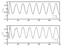
The closed-loop response with $r\left(t\right)=\sin t$ for $t\in\left[0,100\right]$ is shown in Fig. 2. It can be seen that $x\left(t\right)$ eventually tracks $x_{m}\left(t\right)$,but the two signals are initially 180$^{\textrm{o}}$ out of phase due to the control reversal. The signal $\hat{x}\left(t\right)$ approximates $x\left(t\right)$ very well.

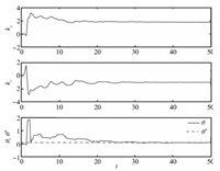
The control parameters $k_{x}\left(t\right)$, $k_{r}\left(t\right)$,and $\theta\left(t\right)$ are shown in Fig. 3. These parameters appear to converge to their ideal values. The convergence is facilitated by having a persistently exciting reference command signal $r\left(t\right)=\sin t$.

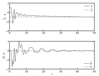
The control input uncertainty $\hat{\lambda}\left(t\right)$ and unmatched disturbance $\hat{w}\left(t\right)$ are estimated as shown in Fig. 4.

Overall,the bi-objective optimal control modification adaptive laws demonstrate good tracking performance.

Remark. Consider an alternate representation of the plant in (1)

\begin{align} \dot{x}=Ax+B\left[u+\Theta^{*{\rm T}}\Phi\left(x\right)\right]+w,\label{1-1} \end{align}

(86)

where $B$ is unknown.

Then,the bi-objective optimal control modification adaptive laws can be recast as

\begin{align} &\dot{K}_{x}^{\rm T}=\Gamma_{x}x\left(e^{\rm T}P+\nu u^{\rm T}\hat{B}^{\rm T}PA_{m}^{-1}\right)\hat{B}, \end{align}

(87)

\begin{align} &\dot{K}_{r}^{\rm T}=\Gamma_{r}r\left(e^{\rm T}P+\nu u^{\rm T}\hat{B}^{\rm T}PA_{m}^{-1}\right)\hat{B}, \end{align}

(88)

\begin{align} &\dot{\Theta}=-\Gamma_{\Theta}\Phi\left(x\right)\biggl(e^{\rm T}P+\nu u^{\rm T}\hat{B}^{\rm T}PA_{m}^{-1}+e_{p}^{\rm T}W-\notag\\ &\qquad \eta\left\{ \left[u+2\Theta^{\rm T}\Phi\left(x\right)\right]^{\rm T}\hat{B}^{\rm T}+\hat{w}^{\rm T}\right\} WA_{m}^{-1}\biggr)\hat{B},\label{eq:-26-2-1-2-1} \end{align}

(89)

\begin{align} &\dot{\hat{B}}^{\rm T}=-\Gamma_{\Lambda}\left[u+\Theta^{\rm T}\Phi\left(x\right)\right]\biggl(e_{p}^{\rm T}W-\notag\\ &\qquad \eta\left\{ \left[u+2\Theta^{\rm T}\Phi\left(x\right)\right]^{\rm T}\hat{B}^{\rm T}+\hat{w}^{\rm T}\right\} WA_{m}^{-1}\biggr), \end{align}

(90)

\begin{align} &\dot{\hat{w}}^{\rm T}=-\gamma_{w}\biggl(e_{p}^{\rm T}W-\notag\\ &\qquad\eta\left\{ \left[u+2\Theta^{\rm T}\Phi\left(x\right)\right]^{\rm T}\hat{B}^{\rm T}+\hat{w}^{\rm T}\right\} WA_{m}^{-1}\biggr), \end{align}

(91)

where $\hat{B}$ is the estimate of $B$.

Ⅲ. FLIGHT CONTROL SIMULATION

Consider a longitudinal pitch dynamic model of an aircraft

\begin{align} &\left[\begin{array}{ccc} mV+\frac{C_{L_{\dot{\alpha}}}\bar{q}S\bar{c}}{2V} & 0 & 0\\ 0 & 1 & 0\\ -\frac{C_{m_{\dot{\alpha}}}\bar{q}S\bar{c}^{2}}{2V} & 0 & I_{yy} \end{array}\right]\left[\begin{array}{c} \dot{\alpha}\\ \dot{\theta}\\ \dot{q} \end{array}\right]=\notag\\ &\left[\begin{array}{ccc} mg\gamma-C_{L_{\alpha}}\bar{q}S & -mg\gamma & mV-\frac{C_{L_{q}}\bar{q}S\bar{c}}{2V}\\ 0 & 0 & 1\\ C_{m_{\alpha}}\bar{q}S\bar{c} & 0 & \frac{C_{m_{q}}\bar{q}S\bar{c}^{2}}{2V} \end{array}\right]\left[\begin{array}{c} \alpha\\ \theta\\ q \end{array}\right]+\notag\\ &\quad \lambda\left[\begin{array}{c} -C_{L_{\delta_{e}}}\\ 0\\ C_{m_{\delta_{e}}} \end{array}\right]\left(\delta_{e}\left(t-t_{d}\right)+\left[\begin{array}{ccc} \theta_{\alpha}^{*} & 0 & \theta_{q}^{*}\end{array}\right]\left[\begin{array}{c} \alpha\\ \theta\\ q \end{array}\right]\right)+ \notag\\ &\quad \left[\begin{array}{c} w_{\alpha}\\ w_{\theta}\\ w_{q} \end{array}\right],\label{eq:-21} \end{align}

(92)

where $t_{d}=50$ ms is a time delay introduced to account for unmodeled dynamics,and $\lambda\in\left[0,1\right]$ is the control input effectiveness,normally equal to 1.

A numerical model for a full-scale generic transport model (GTM) at Mach 0.8 and altitude of 30 000 ft with the flight path angle $\gamma=0$ is given by \begin{align*} &\left[\begin{array}{c} \dot{\alpha}\\ \dot{\theta}\\ \dot{q} \end{array}\right]=\underbrace{\left[\begin{array}{ccc} -0.7018 & 0 & 0.9761\\ 0 & 0 & 1\\ -2.6923 & 0 & -0.7322 \end{array}\right]}_{A}\left[\begin{array}{c} \alpha\\ \theta\\ q \end{array}\right]+\\ &\quad \lambda\underbrace{\left[\begin{array}{c} -0.0573\\ 0\\ -3.5352 \end{array}\right]}_{B}\times\\ &\quad \left(\delta_{e}\left(t-t_{d}\right)+\left[\begin{array}{ccc} \theta_{\alpha}^{*} & 0 & \theta_{q}^{*}\end{array}\right]\left[\begin{array}{c} \alpha\\ \theta\\ q \end{array}\right]\right)+\left[\begin{array}{c} w_{\alpha}\\ w_{\theta}\\ w_{q} \end{array}\right], \end{align*} where the disturbances are given by \[ \left[\begin{array}{c} w_{\alpha}\\ w_{\theta}\\ w_{q} \end{array}\right]=\left[\begin{array}{c} 0.01\sin t-0.05{\rm e}^{-0.1t}\cos2t\\ -0.01\cos4t\\ 0.02{\rm e}^{-0.5t}\sin3t-0.03\sin2t\cos3t \end{array}\right] \]

A desired reference model of the pitch attitude is given by

\begin{align} \ddot{\theta}_{m}\left(t\right)+2\zeta\omega_{n}\dot{\theta}_{m} \left(t\right)+\omega_{n}^{2}\theta_{m}\left(t\right)=\omega_{n}^{2}r\left(t\right), \end{align}

(93)

where $\zeta=0.85$ and $\omega_{n}=1.5$ rad/s are chosen to give a desired handling characteristic.

Let $x=\left[\begin{array}{ccc} \alpha & \theta & q\end{array}\right]^{\rm T}$,$u=\delta_{e}$,$\Theta^{*{\rm T}}=\left[\begin{array}{ccc} \theta_{\alpha}^{*} & 0 & \theta_{q}^{*}\end{array}\right]=\left[\begin{array}{ccc} 0.4 & 0 & -0.3071\end{array}\right]$,and $\lambda=0.5$. The parametric uncertainty $\Theta^{*}$ and the control input uncertainty $\lambda$ result in a short-period mode damping ratio of 0.2418,which is almost half of the nominal short-period mode damping ratio of 0.4045. A nominal controller is designed with $K_{x}=\frac{1}{b_{3}}\left[\begin{array}{ccc} a_{31} & \omega_{n}^{2} & 2\zeta\omega_{n}+a_{33}\end{array}\right]=\left[\begin{array}{ccc} -0.7616 & 0.6365 & 0.5142\end{array}\right]$ and $k_{r}=\frac{1}{b_{3}}\omega_{n}^{2}=-0.6365$. The closed-loop eigenvalues of the ideal plant are $-0.6582$ and $-1.2750\pm0.7902$i. The nominal closed-loop plant is then chosen to be the reference model as \begin{align*} &\underbrace{\left[\begin{array}{c} \dot{\alpha}_{m}\\ \dot{\theta}_{m}\\ \dot{q}_{m} \end{array}\right]}_{\dot{x}_{m}}=\underbrace{\left[\begin{array}{ccc} -0.6582 & -0.0365 & 0.9466\\ 0 & 0 & 1\\ 0 & -2.2500 & -2.5500 \end{array}\right]}_{A_{m}}\times\\ &\quad \underbrace{\left[\begin{array}{c} \alpha_{m}\\ \theta_{m}\\ q_{m} \end{array}\right]}_{x_{m}}+\underbrace{\left[\begin{array}{c} 0.0365\\ 0\\ 2.2500 \end{array}\right]}_{B_{m}}r. \end{align*}

The adaptive controller is given by

\begin{align} u=K_{x}x+k_{r}r+u_{ad},\label{eq:-7} \end{align}

(94)

where $u_{ad}$ is the augmented adaptive control

\begin{align} u_{ad}=\Delta K_{x}\left(t\right)x+\Delta k_{r}\left(t\right)r-\Theta^{\rm T}\left(t\right)x. \end{align}

(95)

Then,$\Delta K_{x}\left(t\right)$,$\Delta k_{r}\left(t\right)$, and $\Theta^{\rm T}\left(t\right)$ are computed from the following bi-objective optimal control modification adaptive laws:

\begin{align} &\Delta\dot{K}_{x}^{\rm T}=\Gamma_{x}x\left(e^{\rm T}P+\nu u_{ad}^{\rm T}\hat{\Lambda}^{\rm T}B^{\rm T}PA_{m}^{-1}\right)B\hat{\Lambda},\label{eq:-16-1-1} \end{align}

(96)

\begin{align} &\Delta\dot{k}_{r}=\gamma_{r}r\left(e^{\rm T}P+\nu u_{ad}^{\rm T}\hat{\Lambda}^{\rm T}B^{\rm T}PA_{m}^{-1}\right)B\hat{\Lambda},\label{eq:-17-1-1} \end{align}

(97)

\begin{align} &\dot{\Theta}=-\Gamma_{\Theta}x\biggl(e^{\rm T}P+\nu u_{ad}^{\rm T}\hat{\Lambda}^{\rm T} B^{\rm T}PA_{m}^{-1}+e_{p}^{\rm T}P-\notag\\ &\qquad \eta\left\{ \left[u+2\Theta^{\rm T}\Phi\left(x\right)\right]^{\rm T}\hat{\Lambda}^{\rm T}B^{\rm T}+\hat{w}^{\rm T}\right\} PA_{m}^{-1}\biggr)B\hat{\Lambda},\label{eq:-20-2} \end{align}

(98)

\begin{align} &\dot{\hat{\Lambda}}^{\rm T}=-\Gamma_{\Lambda}\left[u+\Theta^{\rm T}x\right]\biggl(e_{p}^{\rm T}P-\notag\\ &\qquad \eta\left\{ \left[u+2\Theta^{\rm T}\Phi\left(x\right)\right]^{\rm T}\hat{\Lambda}^{\rm T}B^{\rm T}+\hat{w}^{\rm T}\right\} PA_{m}^{-1}\biggr)B,\label{eq:-20-1-1-1} \end{align}

(99)

\begin{align} &\dot{\hat{w}}^{\rm T}=-\gamma_{w}\biggl(e_{p}^{\rm T}P-\notag\\ &\qquad \eta\left\{ \left[u+2\Theta^{\rm T}\Phi\left(x\right)\right]^{\rm T}\hat{\Lambda}^{\rm T}B^{\rm T}+\hat{w}^{\rm T}\right\} PA_{m}^{-1}\biggr).\label{eq:-6} \end{align}

(100)

These adaptive laws are alternative expressions to those of (29) $\sim$ (33) and (87) $\sim$ (91).

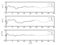
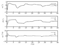
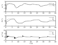
Fig. 5 shows the aircraft response due to the baseline controller. With no adaptation,the closed-loop plant becomes unstable after about 23 s. Fig. 6 is the plot of the aircraft response with the standard MRAC for the adaptive gains $\Gamma_{x}=\Gamma_{\Theta}=\Gamma_{\Lambda}=50 I$ and $\gamma_{r}=50$. The command tracking has improved considerably. However,there is a large initial transient in the pitch rate response as well as high frequency oscillations.

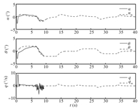
Fig. 7 shows the aircraft response with the bi-objective MRAC by setting $\nu=\eta=0$ in the bi-objective optimal control modification adaptive laws using the same adaptive gains and $\gamma_{w}=50$. The closed-loop becomes unstable after 9 s. The instability of the adaptive laws is consistent with the theory which shows that $\eta$ cannot be zero when an external disturbance $w\left(t\right)$ exists due to the term $c_{8}$ in the stability theorem. Moreover,it is also consistent with the MRAC theory which establishes that the standard MRAC generally exhibits a parameter drift in the presence of a disturbance. To prevent parameter drift, the disturbance estimate $\hat{w}\left(t\right)$ must be bounded by setting $\eta>0$. Alternatively,if the disturbance $w\left(t\right)$ is not estimated by setting $\gamma_{w}=0$,then stability of the bi-objective MRAC will be restored since the term $c_{8}$ becomes bounded for $\eta=0$. Fig. 8 illustrates this observation whereby the aircraft response becomes stable when $\gamma_{w}=0$. Comparing the aircraft response with the bi-objective MRAC with $\gamma_{w}=0$ to that with the standard MRAC,it can be seen that the bi-objective adaptation significantly reduces high frequency oscillations in the pitch rate response.

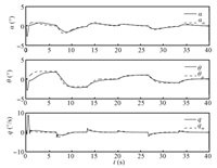
Fig. 9 shows the aircraft response with the bi-objective optimal control modification for the same adaptive gains with $\nu=\eta=0.4$. The pitch rate response is significantly improved with virtually no noticeable large initial transient and high frequency oscillations. However,the pitch attitude tracking is somewhat degraded. This is entirely expected since the bi-objective optimal control modification adaptive laws trade performance for improved robustness. Comparing the aircraft response with the bi-objective MRAC to that with the bi-objective optimal control modification,it can be seen in the pitch rate response that the bi-objective optimal control modification results in smaller initial transients and better tracking.

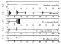
Fig. 10 compares the elevator deflections produced by all the various controllers. The elevator deflection produced by the baseline controller is well within the position limit,but instability still occurs. All adaptive controllers with MRAC exhibit control saturation and high frequency oscillations to varying degrees. The elevator deflection with the standard MRAC exhibits significant high frequency oscillations and control saturation. The elevator deflection with the bi-objective MRAC with $\gamma_{w}>0$ is in full saturation before the controller goes unstable. In contrast,the bi-objective MRAC with $\gamma_{w}=0$ causes only an initial control saturation of the elevator deflection. The amplitude of the control signal then rapidly improves with small periodic transients. In contrast,the bi-objective optimal control modification produces a well-behaved control signal for the elevator deflection with no discernible saturation or high frequency oscillations.

Ⅳ. CONCLUSIONS

This study presents a new method of adaptive control for systems with input uncertainty. A parallel predictor model is constructed to relate the predictor error to the estimation error of the control effectiveness matrix. An optimal control method for a bi-objective cost function to reduce both the tracking error and predictor error simultaneously has been developed. The bi-objective optimal control modification adaptive laws enable the adaptation using both the tracking error and predictor error to improve robustness of the closed-loop systems in the presence of input uncertainty. Simulations show that the bi-objective optimal control modification adaptive laws are quite effective in maintain good tracking performance while improving robustness over the standard model-reference adaptive control.