Classical optimal control problems are formulated in Bernoulli form as the need to find a single control input that minimizes a single cost functional under boundary constraints and dynamical constraints imposed by the system[1, 2]. A multitude of relevant control problems can be modeled as multi-input systems,where each input is computed by a player,and each player attempts to influence the system state to minimize its own cost function. In this case,the optimization problem for each player is coupled with the optimization problem for other players,and hence,in general,an optimal solution in the usual sense does not exist,motivating the formulation of alternative optimality criteria.
Differential game theory provides solution concepts for many multi-player,multi-objective optimization problems[3, 4, 5]. For example,a set of policies is called a Nash equilibrium solution to a multi-objective optimization problem if none of the players can improve their outcomes by changing their policies while all the other players abide by the Nash equilibrium policies[6]. Thus,Nash equilibrium solutions provide a secure set of strategies,in the sense that none of the players have an incentive to diverge from their equilibrium policies. Hence,Nash equilibrium has been a widely used solution concept in differential game-based control techniques.
In general,Nash equilibria are not unique. For a closed-loop differential game (i.e.,the control is a function of the state and time) with perfect information (i.e.,all the players know the complete state history),there can be infinitely many Nash equilibria. If the policies are constrained to be feedback policies,the resulting equilibria are called (sub)game perfect Nash equilibria or feedback-Nash equilibria. The value functions corresponding to feedback-Nash equilibria satisfy a coupled system of Hamilton-Jacobi (HJ) equations[7, 8, 9, 10].
If the system dynamics are nonlinear and uncertain,an analytical solution of the coupled HJ equations is generally infeasible; and hence,dynamic programming-based approximate solutions are sought[11, 12, 13, 14, 15, 16, 17, 18]. In [16],an integral reinforcement learning algorithm is presented to solve nonzero-sum differential games in linear systems without the knowledge of the drift matrix. In [17],a dynamic programming-based technique is developed to find an approximate feedback-Nash equilibrium solution to an infinite horizon $N$-player nonzero-sum differential game online for nonlinear control-affine systems with known dynamics. In [19] ,a policy iteration-based method is used to solve a two-player zero-sum game online for nonlinear control-affine systems without the knowledge of drift dynamics.
The methods in [17] and [19] solve the differential game online using a parametric function approximator such as a neural network (NN) to approximate the value functions. Since the approximate value functions do not satisfy the coupled HJ equations,a set of residual errors (the so-called Bellman errors (BEs)) is computed along the state trajectories and is used to update the estimates of the unknown parameters in the function approximator using least-squares or gradient-based techniques. Similar to adaptive control,a restrictive persistence of excitation (PE) condition is required to ensure boundedness and convergence of the value function weights. Similar to reinforcement learning,an ad-hoc exploration signal is added to the control signal during the learning phase to satisfy the PE condition along the system trajectories[20, 21, 22].
It is unclear how to analytically determine an exploration signal that ensures PE for nonlinear systems; and hence,the exploration signal is typically computed via a simulation-based trial and error approach. Furthermore,the existing online approximate optimal control techniques such as [16, 17, 19, 23] do not consider the ad-hoc signal in the Lyapunov-based analysis. Hence,the stability of the overall closed-loop implementation is not established. These stability concerns,along with concerns that the added probing signal can result in increased control effort and oscillatory transients,provide motivation for the subsequent development.
Based on the ideas in recent concurrent learning-based adaptive control results such as [24] and [25] that show a concurrent learning-based adaptive update law can exploit recorded data to augment the adaptive update laws to establish parameter convergence under conditions milder than PE,this paper extends the work in [17] and [19] to relax the PE condition. In this paper,a concurrent learning-based actor-critic-identifier architecture[23] is used to obtain an approximate feedback-Nash equilibrium solution to an infinite horizon $N$-player nonzero-sum differential game online,without requiring PE,for a nonlinear control-affine system with uncertain linearly parameterized drift dynamics.
A system identifier is used to estimate the unknown parameters in the drift dynamics. The solutions to the coupled HJ equations and the corresponding feedback-Nash equilibrium policies are approximated using parametric universal function approximators. Based on estimates of the unknown drift parameters,estimates for the BEs are evaluated at a set of pre-selected points in the state-space. The value function and the policy weights are updated using a concurrent learning-based least-squares approach to minimize the instantaneous BEs and the BEs evaluated at pre-selected points. Simultaneously,the unknown parameters in the drift dynamics are updated using a history stack of recorded data via a concurrent learning-based gradient descent approach. It is shown that under a condition milder than PE,uniformly ultimately bounded (UUB) convergence of the unknown drift parameters,the value function weights and the policy weights to their true values can be established. Simulation results are presented to demonstrate the performance of the developed technique without an added excitation signal.
II. PROBLEM FORMULATION AND EXACT SOLUTIONConsider a class of control-affine multi-input systems
| \begin{align} \dot{x}=f\left(x\right)+\sum_{i=1}^{N}g_{i}\left(x\right)\hat{u}_{i},\label{eq:Dynamics} \end{align} | (1) |
where $x\in{\bf R} ^{n}$ is the state and $\hat{u}_{i}\in{\bf R} ^{m_{i}}$ are the control inputs (i.e.,the players). In (1),the unknown function $f:{\bf R} ^{n}\to{\bf R} ^{n}$ is linearly parameterizable,the function $g_{i}:{\bf R} ^{n}\to{\bf R} ^{n\times m_{i}}$ is known and uniformly bounded,$f$ and $g_{i}$ are locally Lipschitz,and $f\left(0\right)=0$. Let
\begin{align*} &U:=\{\left\{ u_{i}:{\bf R} ^{n}\to{\bf R} ^{m_{i}},i=1,\cdots ,N\right\} ,\mbox{ such that}\\ &\qquad \mbox{the tuple }\left\{ u_{i},\cdots,u_{N}\right\} \mbox{ is admissible w.r.t. (1)}\} \end{align*}be the set of all admissible tuples of feedback policies. Let $V_{i}^{\left\{ u_{i},\cdots,u_{N}\right\} }:{\bf R} ^{n}\to{\bf R} _{\geq0}$ denote the value function of the $i{\rm th}$ player w.r.t. the tuple of feedback policies $\left\{ u_{1},\cdots,u_{N}\right\} \in U$,defined as
| \begin{align} &V_{i}^{\left\{ u_{1},\cdots,u_{N}\right\} }\left(x\right)=\notag\\ &\qquad \intop\nolimits_{t}^{\infty}r_{i}\left(\phi\left(\tau,x\right),u_{i}\left(\phi\left(\tau,x\right)\right),\cdots, u_{N}\left(\phi\left(\tau,x\right)\right)\right){\rm d}\tau,\label{eq:Vi} \end{align} | (2) |
where $\phi\left(\tau,x\right)$ for $\tau\in[t,\infty)$ denotes the trajectory of (1) obtained using the feedback policies $\hat{u}_{i}\left(\tau\right)=u_{i}\left(\phi\left(\tau,x\right)\right)$ and the initial condition $\phi\left(t,x\right)=x$. In (2),$r_{i}:{\bf R} ^{n}\times{\bf R} ^{m_{1}}\times\cdots\times{\bf R} ^{m_{N}}\to{\bf R} _{\geq0}$ denotes the instantaneous cost defined as $r_{i}\left(x,u_{i},\cdots,u_{N}\right):= x^{\rm T}Q_{i}x+\sum_{j=1}^{N}u_{j}^{\rm T}R_{ij}u_{j}$,where $Q_{i}\in{\bf R} ^{n\times n}$ is a positive definite matrix. The control objective is to find an approximate feedback-Nash equilibrium solution to the infinite horizon regulation differential game online,i.e.,to find a tuple $\left\{ u_{1}^{*},\cdots,u_{N}^{*}\right\} \in U$ such that for all $x \in {{\bf{R}}^n}$,the corresponding value functions satisfy
\begin{align*} V_{i}^{*}\left(x\right)\!:=\! V_{i}^{\left\{ u_{1}^{*},u_{2}^{*},\cdots ,u_{i}^{*},\cdots ,u_{N}^{*}\right\} }\left(x\right)\!\leq\! V_{i}^{\left\{ u_{1}^{*},u_{2}^{*},\cdots,u_{i},\cdots ,u_{N}^{*}\right\} }\left(x\right) \end{align*}for all $u_{i}$ such that $\left\{ u_{1}^{*},u_{2}^{*},\cdots ,u_{i},\cdots,u_{N}^{*}\right\} \in U$.
The exact closed-loop feedback-Nash equilibrium solution $\left\{ u_{i}^{*},\cdots,u_{N}^{*}\right\} $ can be expressed in terms of the value functions as[5, 8, 9, 17]
| \begin{align} u_{i}^{*}=-\frac{1}{2}R_{ii}^{-1}g_{i}^{\rm T}\left(\nabla_{x}V_{i}^{*}\right)^{\rm T}, \end{align} | (3) |
where $\nabla_{x}:=\frac{\partial}{\partial x}$ and the value functions $\left\{ V_{1}^{*},\cdots ,V_{N}^{*}\right\} $ are the solutions to the coupled HJ equations
| \begin{align} &x^{\rm T}Q_{i}x+\sum_{j=1}^{N}\frac{1}{4}\nabla_{x}V_{j}^{*}G_{ij} \left(\nabla_{x}V_{j}^{*}\right)^{\rm T}+\nabla_{x}V_{i}^{*}f-\notag \\ &\qquad \frac{1}{2}\nabla_{x}V_{i}^{*}\sum_{j=1}^{N}G_{j}\left(\nabla_{x}V_{j}^{*}\right)^{\rm T}=0. \end{align} | (4) |
In (4),$G_{j}:= g_{j}R_{jj}^{-1}g_{j}^{\rm T}$ and $G_{ij}:= g_{j}R_{jj}^{-1}R_{ij}R_{jj}^{-1}g_{j}^{\rm T}$. The HJ equations in (4) are in the so-called closed-loop form; they can be expressed in an open-loop form as
| \begin{align} x^{\rm T}Q_{i}x+\sum_{j=1}^{N}u_{j}^{*\rm T}R_{ij}u_{j}^{*}+\nabla_{x}V_{i}^{*}f+\nabla_{x}V_{i}^{*}\sum_{j=1}^{N}g_{j}u_{j}^{*}=0. \end{align} | (5) |
Computation of an analytical solution to the coupled nonlinear HJ equations in (4) is,in general,infeasible. Hence,an approximate solution $\left\{ \hat{V}_{1},\cdots ,\hat{V}_{N}\right\} $ is sought. Based on $\left\{ \hat{V}_{1},\cdots ,\hat{V}_{N}\right\} $,an approximation $\left\{ \hat{u}_{i},\cdots,\hat{u}_{N}\right\} $ to the closed-loop feedback-Nash equilibrium solution is computed. Since the approximate solution,in general,does not satisfy the HJ equations,a set of residual errors (the so-called Bellman errors (BEs)) is computed as
| \begin{align} \delta_{i}=x^{\rm T}Q_{i}x+\sum_{j=1}^{N}\hat{u}_{j}^{\rm T}R_{ij}\hat{u}_{j}+\nabla_{x}\hat{V}_{i}f+\nabla_{x}\hat{V}_{i}\sum_{j=1}^{N}g_{j}\hat{u}_{j}, \end{align} | (6) |
and the approximate solution is recursively improved to drive the BEs to zero. The computation of the BEs in (6) requires knowledge of the drift dynamics $f$. To eliminate this requirement,a concurrent learning-based system identifier is developed in the following section.
A. System IdentificationLet $f\left(x\right)=Y\left(x\right)\theta$ be the linear parametrization of the drift dynamics,where $Y:{\bf R} ^{n}\to{\bf R} ^{n\times p_{\theta}}$ denotes the locally Lipschitz regression matrix,and $\theta\in{\bf R} ^{p_{\theta}}$ denotes the vector of constant,unknown drift parameters. The system identifier is designed as
| \begin{align} \dot{\hat{x}}=Y\left(x\right)\hat{\theta}+\sum_{i=1}^{N}g_{i}\left(x\right)\hat{u}_{i}+k_{x}\tilde{x}, \end{align} | (7) |
where the measurable state estimation error $\tilde{x}$ is defined as $\tilde{x}:= x-\hat{x}$,$k_{x}\in{\bf R} ^{n\times n}$ is a positive definite,constant diagonal observer gain matrix,and $\hat{\theta}\in{\bf R} ^{p_{\theta}}$ denotes the vector of estimates of the unknown drift parameters. In traditional adaptive systems,the estimates are updated to minimize the instantaneous state estimation error,and convergence of parameter estimates to their true values can be established under a restrictive PE condition. In this result,a concurrent learning-based data-driven approach is developed to relax the PE condition to a weaker,verifiable rank condition as follows.
Assumption 1[24, 25]. A history stack $\mathcal{H}_{id}$ containing state-action tuples $\left\{ \left(x_{j},\hat {u}_{1_{j}},\cdots ,\hat {u}_{N_{j}},\right)\mid j=1,\cdots,M_{\theta}\right\} $ recorded along the trajectories of (1) is available a priori,such that
| \begin{align} \mbox{rank}\left(\sum_{j=1}^{M_{\theta}}Y_{j}^{\rm T}Y_{j}\right) & =p_{\theta}, \end{align} | (8) |
where $Y_{j}=Y\left(x_{j}\right)$,and $p_{\theta}$ denotes the number of unknown parameters in the drift dynamics.
To facilitate the concurrent learning-based parameter update,numerical methods are used to compute the state derivative $\dot{x}_{j}$ corresponding to $\left(x_{j},\hat{u}_{j}\right)$. The update law for the drift parameter estimates is designed as
| \begin{align} \dot{\hat{\theta}}=\Gamma_{\theta}Y^{\rm T}\tilde{x}+\Gamma_{\theta}k_{\theta}\sum_{j=1}^{M_{\theta}}Y_{j}^{\rm T}\left(\dot{x}_{j}-\sum_{i=1}^{N}g_{i_{j}}\hat{u}_{i_{j}}-Y_{j}\hat{\theta}\right), \end{align} | (9) |
where $g_{i_{j}}:= g_{i}\left(x_{j}\right)$,$\Gamma_{\theta}\in{\bf R} ^{p\times p}$ is a constant positive definite adaptation gain matrix,and $k_{\theta}\in{\bf R} $ is a constant positive concurrent learning gain. The update law in (9) requires the unmeasurable state derivative $\dot{x}_{j}$. Since the state derivative at a past recorded point on the state trajectory is required,past and future recorded values of the state can be used along with accurate noncausal smoothing techniques to obtain good estimates of $\dot{x}_{j}.$ In the presence of derivative estimation errors,the parameter estimation errors can be shown to be UUB,where the size of the ultimate bound depends on the error in the derivative estimate[24].
To incorporate new information,the history stack is updated with new data. Thus,the resulting closed-loop system is a switched system. To ensure the stability of the switched system,the history stack is updated using a singular value maximizing algorithm[24]. Using (1),the state derivative can be expressed as
\begin{align*} \dot{x}_{j}-\sum_{i=1}^{N}g_{i_{j}}\hat{u}_{i_{j}}=Y_{j}\theta, \end{align*}and hence,the update law in (9) can be expressed in the advantageous form
| \begin{align} \dot{\tilde{\theta}}=-\Gamma_{\theta}Y^{\rm T}\tilde{x}-\Gamma_{\theta}k_{\theta}\left(\sum_{j=1}^{M_{\theta}}Y_{j}^{\rm T}Y_{j}\right)\tilde{\theta}, \end{align} | (10) |
where $\tilde{\theta}:=\theta-\hat{\theta}$ denotes the drift parameter estimation error. The closed-loop dynamics of the state estimation error are given by
| \begin{align} \dot{\tilde{x}}=Y\tilde{\theta}-k_{x}\tilde{x}. \end{align} | (11) |
The value functions,i.e.,the solutions to the HJ equations in (4),are continuously differentiable functions of the state. Using the universal approximation property of NNs,the value functions can be represented as
| \begin{align} V_{i}^{*}\left(x\right)=W_{i}^{\rm T}\sigma_{i}\left(x\right)+\epsilon_{i}\left(x\right), \end{align} | (12) |
where $W_{i}\in{\bf R} ^{p_{W_{i}}}$ denotes the constant vector of unknown NN weights,$\sigma_{i}:{\bf R} ^{n}\to{\bf R} ^{p_{W_{i}}}$ denotes the known NN activation function,$p_{Wi}\in{\bf N}$ denotes the number of hidden layer neurons,and $\epsilon_{i}:{\bf R} ^{n}\to{\bf R} $ denotes the unknown function reconstruction error. The universal function approximation property guarantees that over any compact domain $\mathcal{C}\subset{\bf R} ^{n}$,for all constants $\overline{\epsilon}_{i},\overline{\epsilon}_{i}^{\prime}>0$,there exist a set of weights and basis functions such that $\left\Vert W_{i}\right\Vert \leq\overline{W}$,$\sup_{x\in\mathcal{C}}\left\Vert \sigma_{i}\left(x\right)\right\Vert \leq\overline{\sigma}_{i}$,$\sup_{x\in\mathcal{C}}\left\Vert \sigma_{i}^{\prime}\left(x\right)\right\Vert \leq\overline{\sigma}_{i}^{\prime}$,$\sup_{x\in\mathcal{C}}\left\Vert \epsilon_{i}\left(x\right)\right\Vert \leq\overline{\epsilon}_{i}$ and $\sup_{x\in\mathcal{C}}\left\Vert \epsilon_{i}^{\prime}\left(x\right)\right\Vert \leq\overline{\epsilon}_{i}^{\prime}$,where $\overline{W}_{i},\overline{\sigma}_{i},\overline{\sigma}_{i}^{\prime},\overline{\epsilon}_{i},\overline{\epsilon}_{i}^{\prime}\in{\bf R} $ are positive constants. Based on (3) and (12),the feedback-Nash equilibrium solutions are given by
| \begin{align} u_{i}^{*}\left(x\right)=-\frac{1}{2}R_{ii}^{-1}g_{i}^{\rm {\rm T}}\left(x\right)\left(\sigma_{i}^{\prime {\rm T}}\left(x\right)W_{i}+\epsilon_{i}^{\prime {\rm T}}\left(x\right)\right). \end{align} | (13) |
The NN-based approximations to the value functions and the controllers are defined as
| \begin{align} \hat{V}_{i}:=\hat{W}_{ci}^{\rm T}\sigma_{i},\quad\hat{u}_{i}:=-\frac{1}{2}R_{ii}^{-1}g_{i}^{\rm T}\sigma_{i}^{\prime {\rm T}}\hat{W}_{ai}, \end{align} | (14) |
where $\hat{W}_{ci}\in{\bf R} ^{p_{W_{i}}}$,i.e.,the value function weights,and $\hat{W}_{ai}\in{\bf R} ^{p_{W_{i}}}$,i.e.,the policy weights,are the estimates of the ideal weights $W_{i}$. The use of two different sets of estimates to approximate the same set of ideal weights is motivated by the subsequent stability analysis and the fact that it facilitates an approximate formulation of the BEs which is affine in the value function weights,enabling least squares-based adaptation. Based on (14),measurable approximations to the BEs in (6) are developed as
| \begin{align} \hat{\delta}_{i}=\omega_{i}^{\rm T}\hat{W}_{ci}+x^{\rm T}Q_{i}x+\sum_{j=1}^{N}\frac{1}{4}\hat{W}_{aj}^{\rm T}\sigma_{j}^{\prime}G_{ij}\sigma_{j}^{\prime {\rm T}}\hat{W}_{aj}, \end{align} | (15) |
where $\omega_{i}:=\sigma_{i}^{\prime}Y\hat{\theta}-\frac{1}{2}\sum_{j=1}^{N}\sigma_{i}^{\prime}G_{j}\sigma_{j}^{\prime {\rm T}}\hat{W}_{aj}$. The following assumption,which is generally weaker than the PE assumption,is required for convergence of the concurrent learning-based value function weight estimates.
Assumption 2. For each $i\in\left\{ 1,\cdots,N\right\} $,there exist a finite set of $M_{xi}$ points $\left\{ x_{ij}\in{\bf R} ^{n}\mid j=1,\cdots,M_{xi}\right\} $ such that for all $t\in{\bf R} _{\geq0}$,
| \begin{align} &\mbox{rank}\left(\sum_{k=1}^{M_{xi}}\frac{\omega_{i}^{k} \left(t\right)\left(\omega_{i}^{k}\right)^{\rm T}\left(t\right)}{\rho_{i}^{k}\left(t\right)}\right) =p_{W_{i}},\nonumber \\ &\underline{c}_{xi}\!:=\!\frac{\left(\inf\limits_{t\in{\bf R} _{\geq0}}\left({\lambda}_{\min}\left\{ \sum\limits_{k=1}^{M_{xi}}\frac{\omega_{i}^{k}\left(t\right)\left(\omega_{i}^{k}\right)^{\rm T}\left(t\right)}{\rho_{i}^{k}\left(t\right)}\right\} \right)\right)}{M_{xi}} \!>\!0, \end{align} | (16) |
where $\lambda_{\min}$ denotes the minimum eigenvalue,and $\underline{c}_{xi}\in{\bf R} $ is a positive constant. In (16),$\omega_{i}^{k}\left(t\right):=\sigma_{i}^{\prime ik}Y^{ik}\hat{\theta}\left(t\right)-\frac{1}{2}\sum_{j=1}^{N}\sigma_{i}^{\prime ik}G_{j}^{ik}\left(\sigma_{j}^{\prime ik}\right)^{\rm T}\hat{W}_{aj}\left(t\right)$,where the superscript $ik$ indicates that the term is evaluated at $x=x_{ik}$,and $\rho_{i}^{k}:=1+\nu_{i}\left(\omega_{i}^{k}\right)^{\rm T}\Gamma_{i}\omega_{i}^{k}$,where $\nu_{i}\in{\bf R} _{>0}$ is the normalization gain and $\Gamma_{i}\in{\bf R} ^{P_{W_{i}}\times P_{W_{i}}}$ is the adaptation gain matrix.
The concurrent learning-based least-squares update law for the value function weights is designed as
| \begin{align} &\dot{\hat{W}}_{ci}=-\eta_{c1i}\Gamma_{i}\frac{\omega_{i}}{\rho_{i}}\hat{\delta}_{i}- \frac{\eta_{c2i}\Gamma_{i}}{M_{xi}}\sum_{k=1}^{M_{xi}}\frac{\omega_{i}^{k}}{\rho_{i}^{k}}\hat{\delta}_{i}^{k},\nonumber \\ &\dot{\Gamma}_{i} =\left(\beta_{i}\Gamma_{i}-\eta_{c1i}\Gamma_{i}\frac{\omega_{i}\omega_{i}^{\rm T}}{\rho_{i}^{2}}\Gamma_{i}\right)\mathbf{1}_{\left\{ \left\Vert \Gamma_{i}\right\Vert \leq\overline{\Gamma}_{i}\right\} },\notag \\ &\left\Vert \Gamma_{i}\left(t_{0}\right)\right\Vert \leq\overline{\Gamma}_{i}, \end{align} | (17) |
where $\rho_{i}:=1+\nu_{i}\omega_{i}^{\rm T}\Gamma_{i}\omega_{i}$,$\mathbf{1}_{\left\{ \cdot\right\} }$ denotes the indicator function,$\overline{\Gamma}_{i}>0\in{\bf R} $ is the saturation constant,$\beta_{i}\in{\bf R} $ is the constant positive forgetting factor,$\eta_{c1i},\eta_{c2i}\in{\bf R} $ are constant positive adaptation gains,and the approximate BE $\hat{\delta}_{i}^{k}$ is defined as
\begin{align*} \hat{\delta}_{i}^{k} :=\left(\omega_{i}^{k}\right)^{\rm T}\hat{W}_{ci}+x_{ik}^{\rm T}Q_{i}x_{ik}\!+\!\sum_{j=1}^{N}\frac{\hat{W}_{aj}^{\rm T}\sigma_{j}^{\prime ik}G_{ij}^{ik}\left(\sigma_{j}^{\prime ik}\right)^{\rm T}\hat{W}_{aj}}{4}. \end{align*}The policy weight update laws are designed based on the subsequent stability analysis as
| \begin{align} &\dot{\hat{W}}_{ai}=-\eta_{a1i}\left(\hat{W}_{ai}-\hat{W}_{ci}\right)-\eta_{a2i}\hat{W}_{ai}+\notag\\ &\qquad \frac{1}{4}\sum_{j=1}^{N}\eta_{c1i}\sigma_{j}^{\prime}G_{ij}\sigma_{j}^{\prime {\rm T}}\hat{W}_{aj}^{\rm T} \frac{\omega_{i}^{\rm T}}{\rho_{i}}\hat{W}_{ci}^{\rm T}+\notag\\ &\qquad \frac{1}{4}\sum_{k=1}^{M_{xi}}\sum_{j=1}^{N}\frac{\eta_{c2i}}{M_{xi}}\sigma_{j}^{\prime ik}G_{ij}^{ik}\left(\sigma_{j}^{\prime ik}\right)^{\rm T}\hat{W}_{aj}^{\rm T}\frac{\left(\omega_{i}^{k}\right)^{\rm T}}{\rho_{i}^{k}}\hat{W}_{ci}^{\rm T}, \end{align} | (18) |
where $\eta_{a1i},\eta_{a2i}\in{\bf R} $ are positive constant adaptation gains. The forgetting factor $\beta_{i}$ along with the saturation in the update law for the least-squares gain matrix in (17) ensure that the least-squares gain matrix $\Gamma_{i}$ and its inverse is positive definite and bounded for all $i\in\left\{ 1,\cdots ,N\right\} $ as[26]
| \begin{align} \underline{\Gamma}_{i}\leq\left\Vert \Gamma_{i}\left(t\right)\right\Vert \leq\overline{\Gamma}_{i},\quad \forall t\in{\bf R} _{\geq0}, \end{align} | (19) |
where $\underline{\Gamma}_{i}\in{\bf R} $ is a positive constant,and the normalized regressor is bounded as
\begin{align*} \left\Vert \frac{\omega_{i}}{\rho_{i}}\right\Vert \leq\frac{1}{2\sqrt{\nu_{i}\underline{\Gamma}_{i}}}. \end{align*} IV. STABILITY ANALYSISSubtracting (4) from (15),the approximate BE can be expressed in an unmeasurable form as
\begin{align*} &\hat{\delta}_{i} =\omega_{i}^{\rm T}\hat{W}_{ci}+x^{\rm T}Q_{i}x+\sum_{j=1}^{N}\frac{1}{4}\hat{W}_{aj}^{\rm T} \sigma_{j}^{\prime}G_{ij}\sigma_{j}^{\prime {\rm T}}\hat{W}_{aj}-\\ &\qquad \left(x^{\rm T}Q_{i}x+\sum_{j=1}^{N}u_{j}^{*\rm T}R_{ij}u_{j}^{*}+\nabla_{x}V_{i}^{*}f+\nabla_{x}V_{i}^{*}\sum_{j=1}^{N}g_{j}u_{j}^{*}\right). \end{align*}Substituting for $V^{*}$ and $u^{*}$ from (12) and (13) and using $f=Y\theta$,the approximate BE can be expressed as
\begin{align*} &\hat{\delta}_{i}=\omega_{i}^{\rm T}\hat{W}_{ci}+\sum_{j=1}^{N}\frac{1}{4}\hat{W}_{aj}^{\rm T}\sigma_{j}^{\prime}G_{ij} \sigma_{j}^{\prime {\rm T}}\hat{W}_{aj}-W_{i}^{\rm T}\sigma_{i}^{\prime}Y\theta-\epsilon_{i}^{\prime}Y\theta-\\ &\qquad \sum_{j=1}^{N}\frac{1}{4}\left(W_{j}^{\rm T}\sigma_{j}^{\prime}G_{ij}\sigma_{j}^{\prime {\rm T}}W_{j}+ 2\epsilon_{j}^{\prime}G_{ij}\sigma_{j}^{\prime {\rm T}}W_{j}+\epsilon_{j}^{\prime}G_{ij}\epsilon_{j}^{\prime {\rm T}}\right)\!\!+\\ &\qquad \frac{1}{2}\sum_{j=1}^{N}\left(W_{i}^{\rm T}\sigma_{i}^{\prime}G_{j}\sigma_{j}^{\prime {\rm T}}W_{j}+ \epsilon_{i}^{\prime}G_{j}\sigma_{j}^{\prime {\rm T}}W_{j}+W_{i}^{\rm T}\sigma_{i}^{\prime}G_{j}\epsilon_{j}^{\prime {\rm T}}\right)\!\!+\\ &\qquad \frac{1}{2}\sum_{j=1}^{N}\epsilon_{i}^{\prime}G_{j}\epsilon_{j}^{\prime {\rm T}}. \end{align*}Adding and subtracting $\frac{1}{4}\hat{W}_{aj}^{\rm T}\sigma_{j}^{\prime}G_{ij}\sigma_{j}^{\prime {\rm T}}W_{j}+\omega_{i}^{\rm T}W_{i}$ yields
| \begin{align} &\hat{\delta}_{i} =-\omega_{i}^{\rm T}\tilde{W}_{ci}+\frac{1}{4}\sum_{j=1}^{N}\tilde{W}_{aj}^{\rm T} \sigma_{j}^{\prime}G_{ij}\sigma_{j}^{\prime {\rm T}}\tilde{W}_{aj}-W_{i}^{\rm T} \sigma_{i}^{\prime}Y\tilde{\theta}-\nonumber \\ &\qquad \frac{1}{2}\sum_{j=1}^{N}\left(W_{i}^{\rm T}\sigma_{i}^{\prime}G_{j}-W_{j}^{\rm T}\sigma_{j}^{\prime}G_{ij}\right)\sigma_{j}^{\prime {\rm T}}\tilde{W}_{aj}-\epsilon_{i}^{\prime}Y\theta+\Delta_{i}, \end{align} | (20) |
where $\Delta_{i}:=\frac{1}{2}\sum_{j=1}^{N}\left(W_{i}^{\rm T}\sigma_{i}^{\prime}G_{j}-W_{j}^{\rm T}\sigma_{j}^{\prime}G_{ij}\right)\epsilon_{j}^{\prime {\rm T}}+\frac{1}{2}\sum_{j=1}^{N}W_{j}^{\rm T}\sigma_{j}^{\prime}G_{j}\epsilon_{i}^{\prime {\rm T}}+\frac{1}{2}\sum_{j=1}^{N}\epsilon_{i}^{\prime}G_{j}\epsilon_{j}^{\prime {\rm T}}-\sum_{j=1}^{N}\frac{1}{4}\epsilon_{j}^{\prime}G_{ij}\epsilon_{j}^{\prime {\rm T}}.$ Similarly,the approximate BE evaluated at the selected points can be expressed in an unmeasurable form as
| \begin{align} &\hat{\delta}_{i}^{k} =-\omega_{i}^{k\rm T}\tilde{W}_{ci}+\frac{1}{4}\sum_{j=1}^{N}\tilde{W}_{aj}^{\rm T}\sigma_{j} ^{\prime ik}G_{ij}^{ik}\left(\sigma_{j}^{\prime ik}\right)^{\rm T}\tilde{W}_{aj}+\Delta_{i}^{k}-\nonumber \\ &\qquad \frac{1}{2}\sum_{j=1}^{N}\left(W_{i}^{\rm T}\sigma_{i}^{\prime ik}G_{j}^{ik}-W_{j}^{\rm T}\sigma_{j} ^{\prime ik}G_{ij}^{ik}\right)\left(\sigma_{j}^{\prime ik}\right)^{\rm T}\tilde{W}_{aj}-\nonumber \\ &\qquad W_{i}^{\rm T}\sigma_{i}^{\prime ik}Y^{ik}\tilde{\theta}, \end{align} | (21) |
where the constant $\Delta_{i}^{k}\in{\bf R} $ is defined as $\Delta_{i}^{k}:=-\epsilon_{i}^{\prime ik}Y^{ik}\theta+\Delta_{i}^{ik}$. To facilitate the stability analysis,a candidate Lyapunov function is defined as
| \begin{align} &V_{L} =\sum_{i=1}^{N}V_{i}^{*}+\frac{1}{2}\sum_{i=1}^{N}\tilde{W}_{ci}^{\rm T}\Gamma_{i}^{-1}\tilde{W}_{ci}+ \frac{1}{2}\sum_{i=1}^{N}\tilde{W}_{ai}^{\rm T}\tilde{W}_{ai}+\nonumber \\ & \qquad \frac{1}{2}\tilde{x}^{\rm T}\tilde{x}+\frac{1}{2}\tilde{\theta}^{\rm T}\Gamma_{\theta}^{-1}\tilde{\theta}. \end{align} | (22) |
Since $V_{i}^{*}$ are positive definite,the bound in (19) and Lemma 4.3 in [27] can be used to bound the candidate Lyapunov function as
| \begin{align} \underline{v}\left(\left\Vert Z\right\Vert \right)\leq V_{L}\left(Z,t\right)\leq\overline{v}\left(\left\Vert Z\right\Vert \right), \end{align} | (23) |
where $Z=\left[x^{\rm T},\tilde{W}_{c1}^{\rm T},\cdots,\tilde{W}_{cN}^{\rm T},\tilde{W}_{a1}^{\rm T},\cdots,\tilde{W}_{aN}^{\rm T},\tilde{x},\tilde{\theta}\right]^{\rm T}\in{\bf R} ^{2n+2N\sum_{i}p_{W_{i}}+p_{\theta}}$ and $\underline{v},\overline{v}:{\bf R} _{\geq0}\to{\bf R} _{\geq0}$ are class $\mathcal{K}$ functions. For any compact set $\mathcal{Z}\subset{\bf R} ^{2n+2N\sum_{i}p_{W_{i}}+p_{\theta}},$ define
| \begin{align*} &{\iota _1}:=\max_{i,j}\left(\sup_{Z\in\mathcal{Z}} \left\Vert \frac{1}{2}W_{i}^{\rm T}\sigma_{i}^{\prime}G_{j}\sigma_{j}^{\prime {\rm T}}+ \frac{1}{2}\epsilon_{i}^{\prime}G_{j}\sigma_{j}^{\prime {\rm T}}\right\Vert \right),\notag\\ &{\iota _2}:=\max_{i,j}\Bigl(\sup_{Z\in\mathcal{Z}} \Bigl\Vert\frac{\eta_{c1i}\omega_{i}}{4\rho_{i}} \left(3W_{j}\sigma_{j}^{\prime}G_{ij}-2W_{i}^{\rm T}\sigma_{i}^{\prime}G_{j}\right)\sigma_{j}^{\prime {\rm T}}+\notag\\ &\quad\sum_{k=1}^{M_{xi}}\frac{\eta_{c2i}\omega_{i}^{k}}{4M_{xi}\rho_{i}^{k}}\left(3W_{j}^{\rm T}\sigma_{j}^ {\prime ik}G_{ij}^{ik}-2W_{i}^{\rm T}\sigma_{i}^{\prime ik}G_{j}^{ik}\right)\left(\sigma_{j} ^{\prime ik}\right)^{\rm T}\Bigr\Vert\Bigr),\notag\\ &\iota_{3}:=\max_{i,j}\Bigl(\sup_{Z\in\mathcal{Z}}\Bigl\Vert\frac{1}{2} \sum_{i,j=1}^{N}\left(W_{i}^{\rm T}\sigma_{i}^{\prime}+ \epsilon_{i}^{\prime}\right)G_{j}\epsilon_{j}^{\prime {\rm T}}-\notag\\ &\quad\frac{1}{4}\sum_{i,j=1}^{N}\left(2W_{j}^{\rm T} \sigma_{j}^{\prime}+\epsilon_{j}^{\prime}\right)G_{ij}\epsilon_{j}^{\prime {\rm T}}\Big\Vert\Big),\notag\\ &\iota_{4}:=\max_{i,j}\left(\sup_{Z\in\mathcal{Z}}\left\Vert \sigma_{j}^{\prime}G_{ij}\sigma_{j}^{\prime {\rm T}}\right\Vert \right),\:\iota_{5i}:=\frac{\eta_{c1i}L_{Y}\overline{\epsilon}_{i}^{\prime} \overline{\theta}}{4\sqrt{\nu_{i}\underline{\Gamma}_{i}}},\nonumber \\ &\iota_{6i}:=\frac{\eta_{c1i}L_{Y}\overline{W}_{i} \overline{\sigma}_{i}^{\prime}}{4\sqrt{\nu_{i}\underline{\Gamma}_{i}}},\: \iota_{7i}:=\frac{\eta_{c2i}\max\limits_{k}\left\Vert \sigma_{i}^{\prime ik}Y^{ik}\right \Vert \overline{W}_{i}}{4\sqrt{\nu_{i}\underline{\Gamma}_{i}}},\nonumber \\&{\iota _8}: = \sum\limits_{i = 1}^N {\frac{{\left( {{\eta _{c1i}} + {\eta _{c2i}}} \right){{\bar W}_i}{\iota _4}}}{{8\sqrt {{\nu _i}{{}_i}} }}} ,\:{\iota _{9i}}: = \left( {{\iota _1}N + \left( {{\eta _{a2i}} + {\iota _8}} \right){{\bar W}_i}} \right),\\ &\iota_{10i}:=\frac{\eta_{c1i}\sup\limits_{Z\in\mathcal{Z}}\left\Vert \Delta_{i}\right\Vert +\eta_{c2i}\max\limits_{k}\left\Vert \Delta_{i}^{k}\right\Vert } {2\sqrt{\nu_{i}\underline{\Gamma}_{i}}},\end{align*} \begin{align} &v_{l}:=\sqrt{\frac{1}{2} \min\left(\frac{\underline{q_{i}}}{2},\frac{\eta_{c2i}\underline{c}_{xi}}{4}, \underline{k_{x}},\frac{2\eta_{a1i}+\eta_{a2i}}{8},\frac{k_{\theta}\underline{y}}{2}\right)},\nonumber \\ &\iota:=\sqrt{\sum_{i=1}^{N}\left(\frac{2\iota_{9i}^{2}}{2\eta_{a1i}+\eta_{a2i}}+ \frac{\iota_{10i}^{2}}{\eta_{c2i}\underline{c}_{xi}}\right)+\iota_{3}}, \end{align} | (24) |
where $\underline{y}$ denotes the minimum eigenvalue of $\sum_{j=1}^{ M_{\theta} }Y_{j}^{T}Y_{j}$,$\underline{q_{i}}$ denotes the minimum eigenvalue of $Q_{i}$,$\underline{k_{x}}$ denotes the minimum eigenvalue of $k_{x}$,and the suprema exist since $\frac{\omega_{i}}{\rho_{i}}$ is uniformly bounded for all $Z$,and the functions $G_{i}$,$G_{ij}$,$\sigma_{i}$,and $\epsilon_{i}^{\prime}$ are continuous. In (24),$L_{Y}\in{\bf R} _{\geq0}$ denotes the Lipschitz constant such that $\left\Vert Y\left(\varpi\right)\right\Vert \leq L_{Y}\left\Vert \varpi\right\Vert $ for all $\varpi\in\mathcal{Z}\cap{\bf R} ^{n}.$ The sufficient conditions for UUB convergence are derived based on the subsequent stability analysis as
| \begin{align} &\underline{q_{i}} >2\iota_{5i},\nonumber \\ &\eta_{c2i}\underline{c}_{xi} >2\iota_{5i}+2\zeta_{1}\iota_{7i}+\iota_{2}\zeta_{2}N+\eta_{a1i}+2\zeta_{3}\iota_{6i}\overline{Z},\nonumber \\ &2\eta_{a1i}+\eta_{a2i} >4\iota_{8}+\frac{2\iota_{2}N}{\zeta_{2}},\nonumber \\ &k_{\theta}\underline{y} >\frac{2\iota_{7i}}{\zeta_{1}}+2\frac{\iota_{6i}}{\zeta_{3}}\overline{Z}, \end{align} | (25) |
where $\overline{Z}:=\underline{v}^{-1}\left(\overline{v}\left(\max\left(\left\Vert Z\left(t_{0}\right)\right\Vert ,\frac{\iota}{v_{l}}\right)\right)\right)$ and $\zeta_{1},\zeta_{2},\zeta_{3}\in{\bf R} $ are known positive adjustable constants.
Since the NN function approximation error and the Lipschitz constant $L_{Y}$ depend on the compact set that contains the state trajectories,the compact set needs to be established before the gains can be selected using (25). Based on the subsequent stability analysis,an algorithm is developed to compute the required compact set (denoted by $\mathcal{Z}$) based on the initial conditions. In Algorithm 1,the notation $\left\{ \varpi\right\} _{i}$ for any parameter $\varpi$ denotes the value of $\varpi$ computed in the $i$-th iteration. Since the constants $\iota$ and $v_{l}$ depend on $L_{Y}$ only through the products $L_{Y}\overline{\epsilon}_{i}^{\prime}$ and $L_{Y}\zeta_{3}$,Algorithm 1 ensures that
| \begin{align} \frac{\iota }{{{v_l}}} \le \frac{1}{2}{\rm{diam}}\left( {\rm\mathcal{Z}} \right), \end{align} | (26) |
where diam ($\mathcal{Z}$) denotes the diameter of set $\mathcal{Z}$.

Theorem 1. Provided Assumptions 1~2 hold and the control gains satisfy the sufficient conditions in (25),where the constants in (24) are computed based on the compact set $\mathcal{Z}$ selected using Algorithm 1,the system identifier in (7) along with the adaptive update law in (9),and the controllers in (14) along with the adaptive update laws in (17) and (18) ensure that the state $x$,the state estimation error $\tilde{x}$,the value function weight estimation errors $\tilde{W}_{ci}$ and the policy weight estimation errors $\tilde{W}_{ai}$ are UUB,resulting in UUB convergence of the policies $\hat{u}_{i}$ to the feedback-Nash equilibrium policies $u_{i}^{*}$.
Proof. The derivative of the candidate Lyapunov function in (22) along the trajectories of (1),(10),(11),(17),and (18) is given by
| \begin{align*} &\dot{V}_{L} =\sum_{i=1}^{N}\left(\nabla_{x}V_{i}^{*}\left(f+\sum_{j=1}^{N}g_{j}u_{j}\right)\right)+\tilde{x}^{\rm T}\left(Y\tilde{\theta}-k_{x}\tilde{x}\right)+\notag\\ &\qquad \sum_{i=1}^{N}\tilde{W}_{ci}^{\rm T}\left(\frac{\eta_{c1i}\omega_{i}}{\rho_{i}}\hat{\delta}_{i}+\frac{\eta_{c2i}}{M_{xi}}\sum_{i=1}^{M_{xi}}\frac{\omega_{i}^{k}}{\rho_{i}^{k}}\hat{\delta}_{i}^{k}\right)-\notag\\ & \qquad \frac{1}{2}\sum_{i=1}^{N}\tilde{W}_{ci}^{\rm T}\left(\beta_{i}\Gamma_{i}^{-1}-\eta_{c1i}\frac{\omega_{i}\omega_{i}^{\rm T}}{\rho_{i}^{2}}\right)\tilde{W}_{ci}+\notag\\ & \qquad \tilde{\theta}^{\rm T}\left(-Y^{\rm T}\tilde{x}-k_{\theta}\left(\sum_{j=1}^{M_{\theta}}Y_{j}^{\rm T}Y_{j}\right)\tilde{\theta}\right)- \end{align*} \begin{align} &\qquad \sum_{i=1}^{N}\tilde{W}_{ai}^{\rm T}\Bigg(-\eta_{a1i}\left(\hat{W}_{ai}^{\rm T}-\hat{W}_{ci}^{\rm T}\right)-\eta_{a2i}\hat{W}_{ai}^{\rm T}+\notag\\ &\qquad \frac{1}{4}\sum_{j=1}^{N}\eta_{c1i}\hat{W}_{ci}^{\rm T}\frac{\omega_{i}}{\rho_{i}}\hat{W}_{aj}^{\rm T}\sigma_{j}^{\prime}G_{ij}\sigma_{j}^{\prime {\rm T}}+\notag\\ &\qquad \frac{1}{4}\sum_{k=1}^{M_{xi}}\sum_{j=1}^{N}\frac{\eta_{c2i}}{M_{xi}}\hat{W}_{ci}^{\rm T}\frac{\omega_{i}^{k}}{\rho_{i}^{k}}\hat{W}_{aj}^{\rm T}\sigma_{j}^{\prime ik}G_{ij}^{ik}\left(\sigma_{j}^{\prime ik}\right)^{\rm T}\Bigg). \end{align} | (27) |
Substituting the unmeasurable forms of the BEs from (20) and (21) into (27),and using the triangle inequality,the Cauchy-Schwarz inequality and Young$'$s inequality,the Lyapunov derivative in (27) can be bounded as
| \begin{align*} &\dot{V}\leq-\sum_{i=1}^{N}\frac{\underline{q_{i}}}{2}\left\Vert x\right\Vert ^{2}-\sum_{i=1}^{N}\frac{\eta_{c2i}\underline{c}_{xi}}{2}\left\Vert \tilde{W}_{ci}\right\Vert ^{2}-\underline{k_{x}}\left\Vert \tilde{x}\right\Vert ^{2}-\nonumber \\ & \quad \frac{k_{\theta}\underline{y}}{2}\left\Vert \tilde{\theta}\right\Vert ^{2}-\sum_{i=1}^{N}\left(\frac{2\eta_{a1i}+\eta_{a2i}}{4}\right)\left\Vert \tilde{W}_{ai}\right\Vert ^{2}+\nonumber \\ &\quad \sum_{i=1}^{N}\iota_{9i}\left\Vert \tilde{W}_{ai}\right\Vert +\sum_{i=1}^{N}\iota_{10i}\left\Vert \tilde{W}_{ci}\right\Vert-\sum_{i=1}^{N}\left(\frac{q_{i}}{2}-\iota_{5i}\right)\left\Vert x\right\Vert ^{2}- \end{align*} \begin{align} &\quad \sum_{i=1}^{N}\Bigg(\frac{\eta_{c2i}\underline{c}_{xi}}{2}-\iota_{5i}-\zeta_{1}\iota_{7i}-\frac{1}{2}\iota_{2}\zeta_{2}N-\frac{1}{2}\eta_{a1i}-\nonumber \\ &\quad \zeta_{3}\iota_{6i}\left\Vert x\right\Vert \Bigg)\left\Vert \tilde{W}_{ci}\right\Vert ^{2}+\sum_{i=1}^{N} \left(\frac{k_{\theta}\underline{y}}{2}-\frac{\iota_{7i}}{\zeta_{1}}-\frac{\iota_{6i}}{\zeta_{3}} \left\Vert x\right\Vert \right)\left\Vert \tilde{\theta}_{i}\right\Vert ^{2}\!\!+\nonumber \\ &\quad \sum_{i=1}^{N}\left(\frac{2\eta_{a1i}+\eta_{a2i}}{4}-\iota_{8}-\frac{\iota_{2}N}{2\zeta_{2}}\right)\left\Vert \tilde{W}_{ai}\right\Vert ^{2}+\iota_{3}.\label{eq:VLDot2} \end{align} | (28) |
Provided the sufficient conditions in (25) hold and the conditions
| \begin{align} &\frac{\eta_{c2i}\underline{c}_{xi}}{2} >\iota_{5i}+\zeta_{1}\iota_{7i}+\frac{1}{2}\iota_{2}\zeta_{2}N+\frac{1}{2}\eta_{a1i}+\zeta_{3}\iota_{6i}\left\Vert x\right\Vert ,\nonumber \\ &\frac{k_{\theta}\underline{y}}{2} >\frac{\iota_{7i}}{\zeta_{1}}+\frac{\iota_{6i}}{\zeta_{3}}\left\Vert x\right\Vert\end{align} | (29) |
hold for all $t\in{\bf R}_{\geq 0}$. Completing the squares in (28),the bound on the Lyapunov derivative can be expressed as
| \begin{align} &\dot{V} \leq-\sum_{i=1}^{N}\frac{\underline{q_{i}}}{2}\left\Vert x\right\Vert ^{2}- \sum_{i=1}^{N}\frac{\eta_{c2i}\underline{c}_{xi}}{4}\left\Vert \tilde{W}_{ci}\right \Vert ^{2}-\underline{k_{x}}\left\Vert \tilde{x}\right\Vert ^{2}-\nonumber \\ &\qquad \sum_{i=1}^{N}\left(\frac{2\eta_{a1i}+\eta_{a2i}}{8}\right)\left\Vert \tilde{W}_{ai}\right\Vert ^{2}-\frac{k_{\theta}\underline{y}}{2}\left\Vert \tilde{\theta}\right\Vert ^{2}+\iota\leq\nonumber \\ & \qquad-(v_{l}\left\Vert Z\right\Vert)^2,\quad\forall\left\Vert Z\right\Vert >\frac{\iota}{v_{l}},\: Z\in\mathcal{Z}.\label{eq:VLDot3} \end{align} | (30) |
Using (23),(26),and (30),Theorem 4.18 in [27] can be invoked to conclude that $\lim_{t\to\infty} \sup\left\Vert Z\left(t\right)\right\Vert \leq\underline{v}^{-1}\left(\overline{v}\left(\frac{\iota}{v_{l}}\right)\right).$ Furthermore,the system trajectories are bounded as $\left\Vert Z\left(t\right)\right\Vert \leq\overline{Z}$ for all $t\in{\bf R} _{\geq0}$. Hence,the conditions in (25) are sufficient for the conditions in (29) to hold for all $t\in{\bf R} _{\geq0}$.
The error between the feedback-Nash equilibrium policy and the approximate policy can be expressed as
\begin{align*} \left\Vert u_{i}^{*}-\hat{u}_{i}\right\Vert \leq\frac{1}{2}\left\Vert R_{ii}\right\Vert \overline{g_{i}}\overline{\sigma}_{i}^{\prime}\left(\left\Vert \tilde{W}_{ai}\right\Vert +\bar{\epsilon}_{i}^{\prime}\right), \end{align*}for all $i=1,\cdots,N$,where $\overline{g_{i}}:=\sup_{x}\left\Vert g_{i}\left(x\right)\right\Vert $. Since the weights $\tilde{W}_{ai}$ are UUB,UUB convergence of the approximate policies to the feedback-Nash equilibrium policies is obtained.
Remark 1. The closed-loop system analyzed using the candidate Lyapunov function in (22) is a switched system. The switching happens when the history stack is updated and when the least-squares regression matrices $\Gamma_{i}$ reach their saturation bound. Similar to least squares-based adaptive control[26],(22) can be shown to be a common Lyapunov function for the regression matrix saturation,and the use of a singular value maximizing algorithm to update the history stack ensures that (22) is a common Lyapunov function for the history stack updates[24]. Since (22) is a common Lyapunov function,(23),(26) and (30) establish UUB convergence of the switched system.
V. SIMULATION A. Problem SetupTo portray the performance of the developed approach,the concurrent learning-based adaptive technique is applied to the nonlinear control-affine system[17]
| \begin{align} \dot{x}=f\left(x\right)+g_{1}\left(x\right)u_{1}+g_{2}\left(x\right)u_{2},\label{eq:simdyn} \end{align} | (31) |
where $x\in{\bf R} ^{2}$,$u_{1},u_{2}\in{\bf R} $,and
\begin{align*} &f=\left[\begin{array}{cll} x_{2}-2x_{1}\\ \left(\begin{array}{c} -\frac{1}{2}x_{1}-x_{2}+\frac{1}{4}x_{2}\left(\cos\left(2x_{1}\right)+2\right)^{2}\\ +\frac{1}{4}x_{2}\left(\sin\left(4x_{1}^{2}\right)+2\right)^{2} \end{array}\right) \end{array}\right],\\ &g_{1}=\left[\begin{array}{c} 0\\ \cos\left(2x_{1}\right)+2 \end{array}\right],\: g_{2}=\left[\begin{array}{c} 0\\ \sin\left(4x_{1}^{2}\right)+2 \end{array}\right]. \end{align*}The value function has the structure shown in (2) with the weights $Q_{1}=2Q_{2}=2I_{2}$ and $R_{11}=R_{12}=2R_{21}=2R_{22}=2$,where $I_{2}$ is a $2\times2$ identity matrix. The system identification protocol given in Section III-A and the concurrent learning-based scheme given in Section III-B are implemented simultaneously to provide an approximate online feedback-Nash equilibrium solution to the given nonzero-sum two-player game.
B. Analytical SolutionThe control affine system in (31) is selected for this simulation because it is constructed using the converse HJ approach[28] such that the analytical feedback-Nash equilibrium solution of the nonzero-sum game is
\begin{align*} &V_{1}^{*}=\left[\begin{array}{lll} 0.5\\ 0\\ 1 \end{array}\right]^{\rm T}\left[\begin{array}{c} x_{1}^{2}\\ x_{1}x_{2}\\ x_{2}^{2} \end{array}\right],\\ &V_{2}^{*}=\left[\begin{array}{c} 0.25\\ 0\\ 0.5 \end{array}\right]^{\rm T}\left[\begin{array}{c} x_{1}^{2}\\ x_{1}x_{2}\\ x_{2}^{2} \end{array}\right], \end{align*}and the feedback-Nash equilibrium control policies for Player 1 and Player 2 are
\begin{align*} &u_{1}^{*}=-\frac{1}{2}R_{11}^{-1}g_{1}^{\rm T}\left[\begin{array}{cc} 2x_{1} & 0\\ x_{2} & x_{1}\\ 0 & 2x_{2} \end{array}\right]^{\rm T}\left[\begin{array}{c} 0.5\\ 0\\ 1 \end{array}\right],\\ &u_{2}^{*}=-\frac{1}{2}R_{22}^{-1}g_{2}^{\rm T}\left[\begin{array}{cc} 2x_{1} & 0\\ x_{2} & x_{1}\\ 0 & 2x_{2} \end{array}\right]^{\rm T}\left[\begin{array}{c} 0.25\\ 0\\ 0.5 \end{array}\right]. \end{align*}Since the analytical solution is available,the performance of the developed method can be evaluated by comparing the obtained approximate solution against the analytical solution.
C. Simulation ParametersThe dynamics are linearly parameterized as $f=Y\left(x\right)\theta,$ where
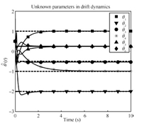
\[ Y\left(x\right)=\left[\begin{array}{lc} x_{2} & 0\\ x_{1} & 0\\ 0 & x_{1}\\ 0 & x_{2}\\ 0 & x_{2}\left(\cos\left(2x_{1}\right)+2\right)^{2}\\ 0 & x_{2}\left(\sin\left(4x_{1}^{2}\right)+2\right)^{2} \end{array}\right]^{\rm T} \]is known and the constant vector of parameters $\theta=\left[1,-2,-\frac{1}{2},-1,\frac{1}{4},-\frac{1}{4}\right]^{\rm T}$ is assumed to be unknown. The initial guess for $\theta$ is selected as $\hat{\theta}\left(t_{0}\right)=0.5\cdot\left[1,1,1,1,1,1\right]^{\rm T}$. The system identification gains are chosen as $k_{x}=5$,$\Gamma_{\theta}=\mbox{diag}\left\{20,20,100,100,60,60\right\}$,$k_{\theta}=1.5$. A history stack of 30 points is selected using a singular value maximizing algorithm[24] for the concurrent learning-based update law in (9),and the state derivatives are estimated using a fifth order Savitzky-Golay filter[29]. Based on the structure of the feedback-Nash equilibrium value functions,the basis function for value function approximation is selected as $\sigma=[x_{1}^{2},x_{1}x_{2},x_{2}^{2}]^{\rm T}$,and the adaptive learning parameters and initial conditions are shown for both players in Tables I and II. Twenty-five points lying on a $5\times5$ grid around the origin are selected for the concurrent learning-based update laws in (17) and (18).
|
|
Table Ⅰ SIMAULATION PARMAMERERS |
|
|
Table Ⅱ SIMULATION INITIAL CONDITIONS |
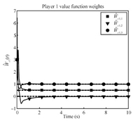
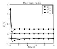
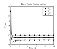
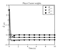
Figs. 1~4 show the rapid convergence of the actor and critic weights to the approximate feedback-Nash equilibrium values for both players,resulting in the value functions and control policies
\begin{align*} \hat{V}_{1}=\left[\begin{array}{clll} 0.5021\\ -0.0159\\ 0.9942 \end{array}\right]^{\rm T}\sigma,\quad\hat{V}_{2}=\left[\begin{array}{c} 0.2510\\ -0.0074\\ 0.4968 \end{array}\right]^{\rm T}\sigma,\\[2mm] \hat{u}_{1}=-\frac{1}{2}R_{11}^{-1}g_{1}^{\rm T}\left[\begin{array}{cc} 2x_{1} & 0\\ x_{2} & x_{1}\\ 0 & 2x_{2} \end{array}\right]^{\rm T}\left[\begin{array}{c} 0.4970\\ -0.0137\\ 0.9810 \end{array}\right],\\[2mm] \hat{u}_{2}=-\frac{1}{2}R_{22}^{-1}g_{2}^{\rm T}\left[\begin{array}{cc} 2x_{1} & 0\\ x_{2} & x_{1}\\ 0 & 2x_{2} \end{array}\right]^{\rm T}\left[\begin{array}{c} 0.2485\\ -0.0055\\ 0.4872 \end{array}\right]. \end{align*}
|
Download:
|
| Fig. 1. Player 1 critic weights convergence. | |
|
Download:
|
| Fig. 2. Player 1 actor weights convergence. | |
|
Download:
|
| Fig. 3. Player 2 critic weights convergence. | |
|
Download:
|
| Fig. 4. Player 2 actor weights convergence. | |
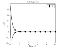
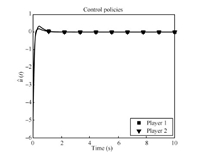
Fig. 5 demonstrates that (without the injection of a PE signal) the system identification parameters also approximately converge to the correct values. The state and control signal trajectories are displayed in Figs. 6 and 7.
|
Download:
|
| Fig. 5. System identification parameters convergence. | |
|
Download:
|
| Fig. 6. State trajectory convergence to the origin. | |
|
Download:
|
| Fig. 7. Control policies of Players 1 and 2. | |
A concurrent learning-based adaptive approach is developed to determine the feedback-Nash equilibrium solution to an $N$-player nonzero-sum game online. The solutions to the associated coupled HJ equations and the corresponding feedback-Nash equilibrium policies are approximated using parametric universal function approximators. Based on estimates of the unknown drift parameters,estimates for the BEs are evaluated at a set of preselected points in the state-space. The value function and the policy weights are updated using a concurrent learning-based least-squares approach to minimize the instantaneous BEs and the BEs evaluated at the preselected points. Simultaneously,the unknown parameters in the drift dynamics are updated using a history stack of recorded data via a concurrent learning-based gradient descent approach.
Unlike traditional approaches that require a restrictive PE condition for convergence,UUB convergence of the drift parameters,the value function and policy weights to their true values,and hence,UUB convergence of the policies to the feedback-Nash equilibrium policies,are established under weaker rank conditions using a Lyapunov-based analysis. Simulations are performed to demonstrate the performance of the developed technique.
The developed result relies on a sufficient condition on the minimum eigenvalue of a time-varying regression matrix. While this condition can be heuristically satisfied by choosing enough points,and can be easily verified online,it cannot,in general,be guaranteed a priori. Furthermore,finding a sufficiently good basis for value function approximation is,in general,nontrivial and can be achieved only through prior knowledge or trial and error. Future research will focus on extending the applicability of the developed technique by relieving the aforementioned shortcomings.
| [1] | Kirk D E. Optimal Control Theory: An Introduction. New York: Dover Publications, 2004. |
| [2] | Lewis F L, Vrabie D, Syrmos V L. Optimal Control (Third edition). New York: John Wiley & Sons, 2012. |
| [3] | Isaacs R. Differential Games: A Mathematical Theory with Applications to Warfare and Pursuit, Control and Optimization. New York: Dover Publications, 1999. |
| [4] | Tijs S. Introduction to Game Theory. Hindustan Book Agency, 2003. |
| [5] | Basar T, Olsder G. Dynamic Noncooperative Game Theory (Second edition). Philadelphia, PA: SIAM, 1999. |
| [6] | Nash J. Non-cooperative games. The Annals of Mathematics, 1951, 54(2): 286-295 |
| [7] | Case J H. Toward a theory of many player differential games. SIAM Journal on Control, 1969, 7(2): 179-197 |
| [8] | Starr A W, Ho C Y. Nonzero-sum differential games. Journal of Optimization Theory and Applications, 1969, 3(3): 184-206 |
| [9] | Starr A, Ho C Y. Further properties of nonzero-sum differential games. Journal of Optimization Theory and Applications, 1969, 3(4): 207-219 |
| [10] | Friedman A. Differential Games. New York: John Wiley and Sons, 1971. |
| [11] | Littman M. Value-function reinforcement learning in Markov games. Cognitive Systems Research, 2001, 2(1): 55-66 |
| [12] | Wei Q L, Zhang H G. A new approach to solve a class of continuoustime nonlinear quadratic zero-sum game using ADP. In: Proceedings of the IEEE International Conference on Networking Sensing and Control. Sanya, China: IEEE, 2008. 507-512 |
| [13] | Vamvoudakis K, Lewis F. Online synchronous policy iteration method for optimal control. In: Proceedings of the Recent Advances in Intelligent Control Systems. London: Springer, 2009. 357-374 |
| [14] | Zhang H G, Wei Q L, Liu D R. An iterative adaptive dynamic programming method for solving a class of nonlinear zero-sum differential games. Automatica, 2010, 47: 207-214 |
| [15] | Zhang X, Zhang H G, Luo Y H, Dong M. Iteration algorithm for solving the optimal strategies of a class of nonaffine nonlinear quadratic zero-sum games. In: Proceedings of the IEEE Conference Decision and Control. Xuzhou, China: IEEE, 2010. 1359-1364 |
| [16] | Vrabie D, Lewis F. Integral reinforcement learning for online computation of feedback Nash strategies of nonzero-sum differential games. In: Proceedings of the 49th IEEE Conference Decision and Control. Atlanta, GA: IEEE, 2010. 3066-3071 |
| [17] | Vamvoudakis K G, Lewis F L. Multi-player non-zero-sum games: online adaptive learning solution of coupled Hamilton-Jacobi equations. Automatica, 2011, 47(8): 1556-1569 |
| [18] | Zhang H, Liu D, Luo Y, Wang D. Adaptive Dynamic Programming for Control-Algorithms and Stability (Communications and Control Engineering). London: Springer-Verlag, 2013 |
| [19] | Johnson M, Bhasin S, Dixon W E. Nonlinear two-player zero-sum game approximate solution using a policy iteration algorithm. In: Proceedings of the 50th IEEE Conference on Decision and Control and European Control Conference. Orlando, FL, USA: IEEE, 2011. 142-147 |
| [20] | Mehta P, Meyn S. Q-learning and pontryagin's minimum principle. In: Proceedings of the IEEE Conference on Decision and Control. Shanghai, China: IEEE, 2009. 3598-3605 |
| [21] | Vrabie D, Abu-Khalaf M, Lewis F L, Wang Y Y. Continuous-time ADP for linear systems with partially unknown dynamics. In: Proceedings of the IEEE International Symposium on Approximate Dynamic Programming and Reinforcement Learning. Honolulu, HI: IEEE, 2007. 247-253 |
| [22] | Sutton R S, Barto A G. Reinforcement Learning: An Introduction. Cambridge, MA, USA: MIT Press, 1998. 4 |
| [23] | Bhasin S, Kamalapurkar R, Johnson M, Vamvoudakis K, Lewis F L, Dixon W. A novel actor-critic-identifier architecture for approximate optimal control of uncertain nonlinear systems. Automatica, 2013, 49(1): 89-92 |
| [24] | Chowdhary G, Yucelen T, Mühlegg M, Johnson E N. Concurrent learning adaptive control of linear systems with exponentially convergent bounds. International Journal of Adaptive Control and Signal Processing, 2012, 27(4): 280-301 |
| [25] | Chowdhary G V, Johnson E N. Theory and flight-test validation of a concurrent-learning adaptive controller. Journal of Guidance, Control, and Dynamics, 2011, 34(2): 592-607 |
| [26] | Ioannou P, Sun J. Robust Adaptive Control. New Jersey: Prentice Hall, 1996. 198 |
| [27] | Khalil H K. Nonlinear Systems (Third edition). New Jersey: Prentice Hall, 2002. 172 |
| [28] | Nevistić V, Primbs J A. Constrained nonlinear optimal control: a converse HJB approach. California Institute of Technology, Pasadena, CA 91125, Techical Report CIT-CDS 96-021, 1996. 5 |
| [29] | Savitzky A, Golay M J E. Smoothing and differentiation of data by simplified least squares procedures. Analytical Chemistry, 1964, 36(8): 1627-1639 |
 2014, Vol.1


